Quickstart

The routines that compute probabilities take a Hamiltonian, as a plain nested list or a NumPy array, and a baseline; the ones that return the evolution operator take the same two. There is no object to construct and no state to configure.

Units

The three core modules are unit-agnostic: they require only that the Hamiltonian and the baseline be given in reciprocal units, so that the product \(H L\) is dimensionless.

Everywhere else in NuOscProbExact the convention is:

Quantity	Units
Hamiltonian	eV
Mass-squared differences	eV²
Neutrino energy	eV
Baseline	eV^-1
Matter potential	eV
Mixing angles, CP phases	radian

globaldefs provides CONV_KM_TO_INV_EV to convert a baseline in km into eV^-1.

An arbitrary Hamiltonian

The shortest possible use: hand the code a Hermitian matrix and a baseline.

import oscprob3nu

hamiltonian = [
    [1.0+0.0j, 0.0+2.0j, 0.0-1.0j],
    [0.0-2.0j, 3.0+0.0j, 3.0+0.0j],
    [0.0+1.0j, 3.0-0.0j, -5.0+0.0j],
]

Pee, Pem, Pet, Pme, Pmm, Pmt, Pte, Ptm, Ptt = \
    oscprob3nu.probabilities_3nu(hamiltonian, 1.0)

print('Pee = %.5f, Pem = %.5f, Pet = %.5f' % (Pee, Pem, Pet))

Pee = 0.54465, Pem = 0.37436, Pet = 0.08099

The probabilities are ordered with the initial flavor varying slowest, so Pem is \(P(\nu_e \to \nu_\mu)\).

The Hamiltonian must be Hermitian, and is checked: one that is not raises ValueError rather than returning numbers, because the numbers it would return still sum to one and so would betray nothing. See oscprob3nu.CHECK_HERMITICITY for the cost of that check and how to decline it. The trace is discarded, since it contributes only an overall phase that cancels in the probabilities.

Oscillations in vacuum

import numpy as np
import oscprob3nu
import hamiltonians3nu
from globaldefs import *

energy = 1.e9      # [eV]
baseline = 1.3e3   # [km]

h_vacuum_energy_indep = \
    hamiltonians3nu.hamiltonian_3nu_vacuum_energy_independent(
        S12_NO_BF, S23_NO_BF, S13_NO_BF, DCP_NO_BF, D21_NO_BF, D31_NO_BF)
h_vacuum = np.multiply(1./energy, h_vacuum_energy_indep)

Pee, Pem, Pet, Pme, Pmm, Pmt, Pte, Ptm, Ptt = \
    oscprob3nu.probabilities_3nu(h_vacuum, baseline*CONV_KM_TO_INV_EV)

print('Pee = %.5f, Pem = %.5f, Pet = %.5f' % (Pee, Pem, Pet))
print('Pme = %.5f, Pmm = %.5f, Pmt = %.5f' % (Pme, Pmm, Pmt))
print('Pte = %.5f, Ptm = %.5f, Ptt = %.5f' % (Pte, Ptm, Ptt))

Pee = 0.92768, Pem = 0.01432, Pet = 0.05800
Pme = 0.04023, Pmm = 0.37887, Pmt = 0.58090
Pte = 0.03210, Ptm = 0.60680, Ptt = 0.36110

hamiltonian_3nu_vacuum_energy_independent deliberately leaves out the factor \(1/E\), so that the energy-independent part can be computed once and reused across an energy scan.

Matter, NSI, and LIV

The remaining sample Hamiltonians all take that same energy-independent vacuum term and add to it:

# Matter of constant density
h_matter = hamiltonians3nu.hamiltonian_3nu_matter(
    h_vacuum_energy_indep, energy, VCC_EARTH_CRUST)

# Non-standard interactions
h_nsi = hamiltonians3nu.hamiltonian_3nu_nsi(
    h_vacuum_energy_indep, energy, VCC_EARTH_CRUST, EPS_3)

# Lorentz invariance-violating background
h_liv = hamiltonians3nu.hamiltonian_3nu_liv(
    h_vacuum_energy_indep, energy, SXI12, SXI23, SXI13, DXICP,
    B1, B2, B3, LAMBDA)

The matter potential VCC is positive for neutrinos. Pass its negative for antineutrinos; see Sign conventions for why that is the whole difference.

Two flavors

oscprob2nu mirrors oscprob3nu throughout:

import oscprob2nu
import hamiltonians2nu

# `sth` is sin(theta), not the angle itself
h2_vacuum_energy_indep = \
    hamiltonians2nu.hamiltonian_2nu_vacuum_energy_independent(
        S23_NO_BF, D31_NO_BF)
h2_vacuum = np.multiply(1./energy, h2_vacuum_energy_indep)

Pee, Pem, Pme, Pmm = \
    oscprob2nu.probabilities_2nu(h2_vacuum, baseline*CONV_KM_TO_INV_EV)

print('Pee = %.5f, Pem = %.5f' % (Pee, Pem))

Pee = 0.29595, Pem = 0.70405

Four flavors

oscprob4nu mirrors the other two in turn, with a \(4\times4\) Hamiltonian and sixteen probabilities. With the fourth state read as sterile, the flavor order is \((\nu_e, \nu_\mu, \nu_\tau, \nu_s)\):

import oscprob4nu
import hamiltonians4nu

# Three extra mixing angles and one extra splitting, here
# Dm41^2 = 1 eV^2.  As everywhere, the angles are given as sines.
h4_vacuum_energy_indep = \
    hamiltonians4nu.hamiltonian_4nu_vacuum_energy_independent(
        S12_NO_BF, S23_NO_BF, S13_NO_BF,
        np.sqrt(0.10), np.sqrt(0.10), 0.0,
        DCP_NO_BF, D21_NO_BF, D31_NO_BF, 1.0)
h4_vacuum = np.multiply(1./energy, h4_vacuum_energy_indep)

prob = oscprob4nu.probabilities_4nu(h4_vacuum,
                                    baseline*CONV_KM_TO_INV_EV)

print('%d probabilities' % len(prob))
print('Pee = %.5f, Pes = %.5f' % (prob[0], prob[3]))
print('they sum to %.5f' % sum(prob[0:4]))

16 probabilities
Pee = 0.76700, Pes = 0.17931
they sum to 1.00000

A sterile state does not feel the neutral-current potential, so that potential no longer cancels between the flavors: in matter it leaves \(-V_{NC}\) on the sterile entry, which is what places the sterile matter resonance. hamiltonians4nu.hamiltonian_4nu_matter() takes both potentials for that reason.

h4_matter = hamiltonians4nu.hamiltonian_4nu_matter(
    h4_vacuum_energy_indep, energy, VCC_EARTH_CRUST, VNC_EARTH_CRUST)

print('sterile entry: %+.4e eV' % h4_matter[3][3].real)

sterile entry: +4.0511e-10 eV

Layered matter and the Earth work at four flavors too — slabs.probabilities_4nu_slabs() and earth.probabilities_4nu_earth() — which is what a 3+1 scenario needs to be propagated through PREM rather than through a single average density.

The evolution operator

If you need the evolution operator itself — to compose it across segments, or to propagate a density matrix — ask for it directly:

U3 = oscprob3nu.evolution_operator_3nu(h_vacuum,
                                       baseline*CONV_KM_TO_INV_EV)

print('|U3[0][0]| = %.6f' % abs(U3[0][0]))

|U3[0][0]| = 0.963160

and the expansion coefficients, if you want those:

h_coeffs = oscprob3nu.hamiltonian_3nu_coefficients(h_vacuum)
u_coeffs = oscprob3nu.evolution_operator_3nu_u_coefficients(
    h_vacuum, baseline*CONV_KM_TO_INV_EV)

print('h has %d coefficients' % len(h_coeffs))

h has 8 coefficients

Because \(H\) is time-independent, the evolution operator obeys the group property \(U(L_1+L_2) = U(L_2) U(L_1)\), which is what makes composing across segments of constant density legitimate.

Layered matter: slabs

A slab is a stretch of the trajectory over which the density is taken constant. slabs solves each one exactly and multiplies the resulting operators together, so the only approximation anywhere is the caller’s — how finely to cut a profile that really varies continuously. Within a slab there is none.

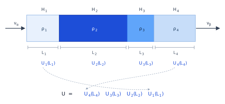
Four slabs of differing width and density, each contributing an evolution operator, multiplied into one operator for the whole trajectory — Each slab carries its own density, and so its own Hamiltonian and its own exactly-solved \(U_k\). The dashed ties are the point of the ordering: the slab crossed *first* is the *rightmost* factor.

Give it one Hamiltonian per slab and one width per slab:

import earth
import slabs

# A denser layer between two lighter ones
densities = [3.0, 5.0, 3.0]                                # [g cm^-3]
widths = np.array([1000.0, 2000.0, 1000.0])*CONV_KM_TO_INV_EV

h_layers = hamiltonians3nu.hamiltonian_3nu_matter(
    h_vacuum_energy_indep, energy, earth.matter_potential(densities))

prob = slabs.probabilities_3nu_slabs(h_layers, widths)

print('h_layers has shape', np.shape(h_layers))
print('P_mue across the three layers = %.6f' % prob[3])

h_layers has shape (3, 3, 3)
P_mue across the three layers = 0.138932

Both arguments are ordered along the trajectory, and the slab met first is applied first — rightmost in \(U = U_n \cdots U_2 U_1\), since the operators act to the left on the initial state. The widths are baselines like any other, so they are in eV^-1, which is what CONV_KM_TO_INV_EV is doing there.

The group property quoted just above is what licenses all of this, and it is visible directly: cutting a uniform profile into slabs must change nothing.

uniform = hamiltonians3nu.hamiltonian_3nu_matter(
    h_vacuum_energy_indep, energy, VCC_EARTH_CRUST)
total = 4000.0*CONV_KM_TO_INV_EV

one_call = oscprob3nu.probabilities_3nu(uniform, total)
split = slabs.probabilities_3nu_slabs(np.stack([uniform]*4),
                                      np.full(4, total/4))

print('one call   %.9f' % one_call[3])
print('four slabs %.9f' % split[3])

one call   0.133015739
four slabs 0.133015739

The two differ by \(6 \times 10^{-16}\) here, and by \(1 \times 10^{-14}\) if the same 4000 km is cut into forty slabs instead: round-off in the extra matrix products, and nothing else.

For the Earth you need not build the slabs at all — earth cuts a chord into PREM layers for you. For the case where the arrangement of the matter, and not merely its mean, is what changes the answer, see “An arbitrary matter profile” in Numerical recipes. Two and four flavors work the same way, through slabs.probabilities_2nu_slabs() and slabs.probabilities_4nu_slabs().

Scanning: pass arrays

probabilities_3nu and evolution_operator_3nu — and their two- and four-flavor counterparts — accept a stack of Hamiltonians, a stack of baselines, or both, and evaluate the whole stack at once. The routines that return expansion coefficients are scalar-only; they are diagnostics rather than the path a scan takes. This is between one and two orders of magnitude faster than the same calls in a Python loop, and it is the recommended way to produce a curve or a grid.

Versus baseline — one Hamiltonian, many baselines:

baselines = np.linspace(1.0, 1.3e4, 2000)*CONV_KM_TO_INV_EV
prob = oscprob3nu.probabilities_3nu(h_vacuum, baselines)

Pem = prob[:, 1]           # same ordering as the scalar return
print('shape:', prob.shape)

shape: (2000, 9)

The characteristic equation depends only on the Hamiltonian, so it is solved once for the whole scan rather than once per baseline.

Versus energy — many Hamiltonians, one baseline. Since \(H \propto 1/E\), build the stack by dividing the energy-independent term by an array of energies:

energies = np.logspace(-1, 1, 2000)*1.e9                  # [eV]
h_stack = h_vacuum_energy_indep/energies[:, None, None]
prob = oscprob3nu.probabilities_3nu(h_stack, baseline*CONV_KM_TO_INV_EV)

print('shape:', prob.shape)

shape: (2000, 9)

The sample Hamiltonians do this for you: pass an array of energies and they return one Hamiltonian per energy, in exactly that shape.

h_stack = hamiltonians3nu.hamiltonian_3nu_matter(
    h_vacuum_energy_indep, energies, VCC_EARTH_CRUST)
prob = oscprob3nu.probabilities_3nu(h_stack, baseline*CONV_KM_TO_INV_EV)

print('shape:', prob.shape)

shape: (2000, 9)

so a whole scan in matter, with NSI, or with LIV is two calls and no Python loop. The matter potential may be an array too, for a scan across a density profile alongside the energy.

An oscillogram is the outer combination of the two: give the Hamiltonians and the baselines separate axes and let them broadcast.

prob = oscprob3nu.probabilities_3nu(h_stack[:, None, :, :],
                                    baselines[:200][None, :])

print('shape:', prob.shape)   # (energies, baselines, 9)

shape: (2000, 200, 9)

A single Hamiltonian and a scalar baseline still return a plain tuple, exactly as before, so existing code is unaffected.

Going faster still

If Numba is installed, the batched paths are evaluated by compiled kernels instead of NumPy, which is worth roughly 1.5x to 20x on large stacks, depending on the number of flavors:

pip install "nuoscprobexact[fast]"

Nothing in your code changes; fastkernels is picked up automatically, and the answers are the same to round-off. If it is not installed, the NumPy path is used and everything works as before.

It is used only where it is faster. For three flavors that is every stack size, by between two and sixteen times, and for four flavors likewise, by between five and nineteen; for two flavors the NumPy path is already lean enough to win below about fifty thousand elements, so it is kept there. fastkernels.worthwhile() makes that choice from measured thresholds, so installing the extra can only help.

Checking the input has a cost too, and it is the larger of the two on a big scan. Every entry point verifies that the Hamiltonian is Hermitian, because one that is not returns probabilities that still sum to one and so betrays nothing. That check is a pass over the stack, the same order of work as evaluating it: 1.3x to 1.8x on a 2000-point scan and 3.2x to 5.7x on a 200 000-point one. Where the Hamiltonians come from a trusted construction, decline it with

import oscprob3nu
oscprob3nu.CHECK_HERMITICITY = False

and likewise for oscprob2nu and oscprob4nu. Everything hamiltonians3nu and its siblings build is Hermitian to round-off.

The first call compiles, which takes a few seconds. The kernels are cached on disk, so later runs start in milliseconds. To force the NumPy path — to compare the two, say — set

import fastkernels
fastkernels.USE_NUMBA = False

The scalar path is deliberately left uncompiled: a single probability takes about eight microseconds, which is not worth a compilation pause. At two and three flavors short stacks are also evaluated one element at a time, since below thirteen elements at three flavors, and twelve at two, the array machinery costs more than it saves; four flavors has no such shortcut, because it has no separate scalar closed form to fall back to.

More examples

The examples/ directory holds a runnable script for each of the cases above, each printing the probabilities it computes. The README walks through the first of them and links the rest, rather than transcribing them, so that there is one copy of each to keep correct.

Note

This directory was called test/ in version 1.0.0 of the code, and is named that way in version 2 of the paper. It was renamed to examples/ to stop it being confused with tests/, which holds the regression suite.