Numerical recipes

What NuOscProbExact can compute, with the code that computes it.

Each recipe below is a few lines and a figure. The figures are the ones the notebooks produce, so the code shown here and the notebook linked beside it are the same calculation — there is no third version to drift out of step. Where a recipe is short enough to be worth running on the spot, it is executed when this page is built and its output is what you see.

One probability

The shortest useful thing the library does. Give it a Hermitian matrix and a baseline in reciprocal units, and it returns the exact probabilities.

import numpy as np

import globaldefs as gd
import hamiltonians3nu
import oscprob3nu

KM = gd.CONV_KM_TO_INV_EV
GEV = 1.0e9

h_vacuum = hamiltonians3nu.hamiltonian_3nu_vacuum_energy_independent(
    gd.S12_NO_BF, gd.S23_NO_BF, gd.S13_NO_BF, gd.DCP_NO_BF,
    gd.D21_NO_BF, gd.D31_NO_BF)

prob = oscprob3nu.probabilities_3nu(
    np.asarray(h_vacuum)/(1.0*GEV), 1300.0*KM)

print('P_ee   = %.6f' % prob[0])
print('P_emu  = %.6f' % prob[1])
print('P_etau = %.6f' % prob[2])

P_ee   = 0.927678
P_emu  = 0.014323
P_etau = 0.057999

The nine probabilities come back with the initial flavor varying slowest. Full walk-through: notebook 01.

Giving the mixing angles

Every routine that takes mixing angles takes them as sines by default, which is what globaldefs carries: S12_NO_BF is \(\sin\theta_{12} = 0.5568\), not \(\sin^2\theta_{12} = 0.310\).

That default is a trap for anyone reading from a global fit, because fits publish the squares. Typing the published \(0.310\) under the default is not an error — it is a perfectly good sine, of a different angle — so nothing complains and the answer is quietly wrong. Pass angles= and the published numbers can be typed as printed:

import math

import hamiltonians3nu

# NuFit 4.0, normal ordering, as published
from_sin2 = hamiltonians3nu.hamiltonian_3nu_vacuum_energy_independent(
    0.310, 0.582, 0.02240, gd.DCP_NO_BF, gd.D21_NO_BF, gd.D31_NO_BF,
    angles='sin2')

# The same angles in degrees, phase included
from_deg = hamiltonians3nu.hamiltonian_3nu_vacuum_energy_independent(
    33.83, 49.72, 8.61, 217.0, gd.D21_NO_BF, gd.D31_NO_BF,
    angles='deg')

# And what globaldefs carries, which is the default
from_sin = hamiltonians3nu.hamiltonian_3nu_vacuum_energy_independent(
    gd.S12_NO_BF, gd.S23_NO_BF, gd.S13_NO_BF, gd.DCP_NO_BF,
    gd.D21_NO_BF, gd.D31_NO_BF)

print('sin2 vs sin: %.1e' % abs(from_sin2 - from_sin).max())
print('deg  vs sin: %.1e' % abs(from_deg - from_sin).max())

sin2 vs sin: 0.0e+00
deg  vs sin: 4.0e-08

The four conventions are 'sin', 'sin2', 'rad' and 'deg'. A CP-violating phase has no sine to pass, so it stays in radians under the first two and follows the angles under the last two — which is why the degrees example above gives \(\delta_{\rm CP}\) as 217.0.

Out-of-range values are refused per convention: angles='sin2' rejects anything outside \([0, 1]\), 'sin' anything outside \([-1, 1]\). Neither can catch radians passed under the default, since those are legal sines; that is what the keyword is for.

A scan, without a loop

Pass an array and the whole scan is one call. This is the single most useful thing to know about using the library well.

energies = np.logspace(-1.0, 1.5, 500)*GEV
stack = np.asarray(h_vacuum)/energies[:, None, None]

probabilities = oscprob3nu.probabilities_3nu(stack, 1300.0*KM)

print('shape returned:', probabilities.shape)
print('P_mue at the first three energies:',
      np.round(probabilities[:3, 3], 6))

shape returned: (500, 9)
P_mue at the first three energies: [0.208266 0.30167  0.402009]

Note the shape: a batched call returns (..., 9), with the flavor index last, so probabilities[:, 3] is \(P_{\mu e}\) along the scan. A scalar call returns a tuple of nine instead.

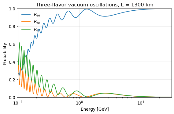
Vacuum oscillations at a 1300 km baseline. Code: notebook 02.

Matter, and new physics

Matter, non-standard interactions and Lorentz-invariance violation are not special cases in the code. Each is a different Hermitian matrix handed to the same routine.

h_matter = hamiltonians3nu.hamiltonian_3nu_matter(
    h_vacuum, energies, gd.VCC_EARTH_CRUST)
h_nsi = hamiltonians3nu.hamiltonian_3nu_nsi(
    h_vacuum, energies, gd.VCC_EARTH_CRUST, gd.EPS_3)

p_matter = oscprob3nu.probabilities_3nu(h_matter, 1300.0*KM)
p_nsi = oscprob3nu.probabilities_3nu(h_nsi, 1300.0*KM)

print('largest difference NSI vs standard matter: %.4f'
      % np.max(np.abs(p_nsi[:, 3] - p_matter[:, 3])))

largest difference NSI vs standard matter: 0.0600

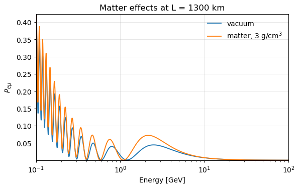
The MSW resonance in constant-density matter. Code: notebook 03.

An oscillogram

A two-dimensional map of energy against baseline, in one call. Index the two arguments so they broadcast against each other and the grid falls out.

n_e, n_l = 240, 240
energies = np.logspace(-1.0, 1.5, n_e)*GEV
baselines = np.linspace(50.0, 12000.0, n_l)*KM

h_stack = hamiltonians3nu.hamiltonian_3nu_matter(
    h_vacuum, energies, gd.VCC_EARTH_CRUST)

# (n_e, 1, 3, 3) against (1, n_l) -> an (n_e, n_l) grid
grid = oscprob3nu.probabilities_3nu(h_stack[:, None, :, :],
                                    baselines[None, :])[:, :, 3]

print('grid shape:', grid.shape, '--', grid.size, 'probabilities')
print('P_mue runs from %.4f to %.4f' % (grid.min(), grid.max()))

grid shape: (240, 240) -- 57600 probabilities
P_mue runs from 0.0000 to 0.5822

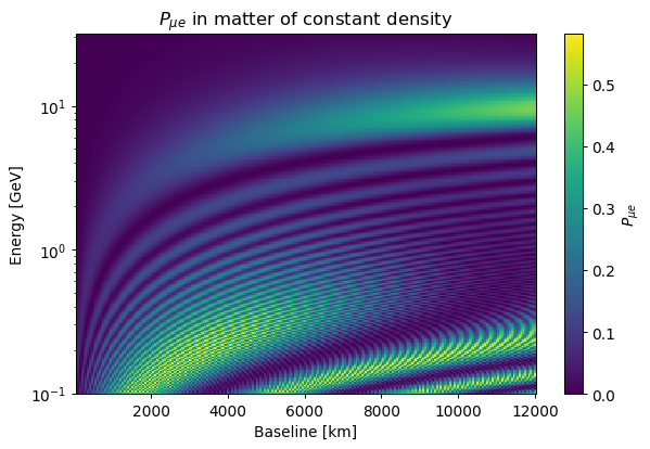
57 600 probabilities, one call, no Python loop. Code: notebook 04.

CP violation

Plotting the neutrino appearance probability against the antineutrino one, as \(\delta_{CP}\) runs through \(2\pi\), traces an ellipse. Matter pushes it off the diagonal, which is what makes the measurement hard.

Antineutrinos need both changes: conjugate the vacuum Hamiltonian and reverse the sign of the potential.

h_nu = hamiltonians3nu.hamiltonian_3nu_matter(
    h_vacuum, 1.0*GEV, gd.VCC_EARTH_CRUST)
h_nubar = hamiltonians3nu.hamiltonian_3nu_matter(
    np.conj(h_vacuum), 1.0*GEV, -gd.VCC_EARTH_CRUST)

print('P(numu -> nue)       = %.6f'
      % oscprob3nu.probabilities_3nu(h_nu, 1300.0*KM)[3])
print('P(numubar -> nuebar) = %.6f'
      % oscprob3nu.probabilities_3nu(h_nubar, 1300.0*KM)[3])

P(numu -> nue)       = 0.025898
P(numubar -> nuebar) = 0.018414

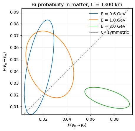
Bi-probability ellipses in matter. Code: notebook 05, and notebook 13 for antineutrinos in full.

Through the Earth

The Earth’s density is not constant, so the expansions do not apply to a whole trajectory. They apply to any piece of it over which the density is taken constant, which is what earth builds from the Preliminary Reference Earth Model [DA81].

import earth

print('chord at costhz = -1 : %.0f km'
      % earth.distance_traveled_inside_earth(-1.0))
print('density at the centre: %.4f g/cm^3' % earth.density_prem(0.0))

probabilities = earth.probabilities_3nu_earth(
    h_vacuum, 8.0*GEV, -0.8, n_slabs_per_segment=6)
print('P_mumu at 8 GeV, costhz = -0.8: %.6f' % probabilities[4])

chord at costhz = -1 : 12742 km
density at the centre: 13.0885 g/cm^3
P_mumu at 8 GeV, costhz = -0.8: 0.527807

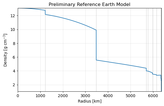
The Preliminary Reference Earth Model. Code: notebook 06.

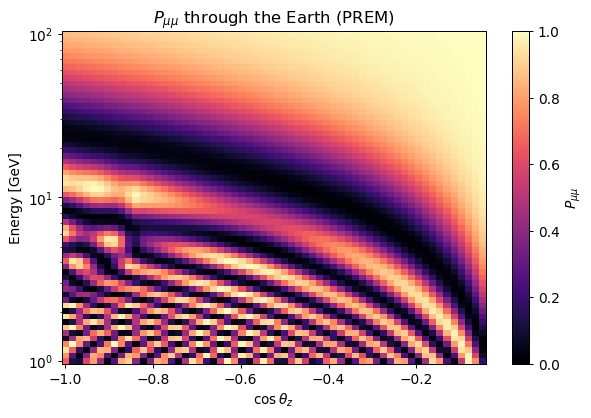
An Earth oscillogram, in energy and zenith angle. Code: notebook 07.

The electron fraction inside the Earth

PREM is a density model: it fixes \(\rho\), not what the rock is made of, so the electron fraction \(Y_e\) has to come from somewhere else. The routines above take one half throughout, which is exactly isoscalar matter and is what no layer of the Earth actually is. earth.electron_fraction_prem() gives the composition of each layer. Pass the function itself, not its values: it is then evaluated at whatever slabs are cut, which is what lets it work with a tolerance.

costhz = -1.0

uniform = earth.probabilities_3nu_earth(
    h_vacuum, 2.0*GEV, costhz, atol=1.0e-5)
layered = earth.probabilities_3nu_earth(
    h_vacuum, 2.0*GEV, costhz, atol=1.0e-5,
    electron_fraction=earth.electron_fraction_prem)

print('P_mue   one half: %.6f   layered: %.6f' % (uniform[3], layered[3]))

P_mue   one half: 0.133572   layered: 0.119698

earth.earth_slab_radii() gives the radii of a chord’s slabs, in the order they come in, for inspecting the profile or building an array by hand. An array works only at a fixed n_slabs_per_segment, since a tolerance chooses the count itself and an array cannot follow it.

radii = earth.earth_slab_radii(costhz, 6)
y_e = earth.electron_fraction_prem(radii)

print('Y_e runs from %.4f to %.4f over %d slabs'
      % (y_e.min(), y_e.max(), len(y_e)))

Y_e runs from 0.4656 to 0.5551 over 114 slabs

The difference is not cosmetic. Through the diameter it is order unity; through the mantle alone a few percent; on a shallow chord well under one. The layers, and the radii that separate them, are:

Layer	Radius (km)	\(Y_e\)	Composition
Core	\(r \leq 3480\)	0.4656	Iron, \(26/55.845\)
Mantle	\(3480 < r \leq 6346.6\)	0.4957	Peridotite
Crust	\(6346.6 < r \leq 6368\)	0.4952	Granitic
Ocean	\(r > 6368\)	0.5551	Seawater, \(10/18.015\)

Every one of the four is a keyword, so any of them may be replaced. The ocean is the one to watch: PREM carries a global average, and a chord that ends at a detector under rock crosses none of it, so pass the crust’s value for a land baseline.

def land_electron_fraction(r):
    return earth.electron_fraction_prem(
        r, ocean=gd.ELECTRON_FRACTION_EARTH_CRUST_LAYER)

land = land_electron_fraction(radii)

print('ocean slabs, as PREM has them: %d'
      % int((y_e == gd.ELECTRON_FRACTION_EARTH_OCEAN).sum()))
print('after replacing them:          %d'
      % int((land == gd.ELECTRON_FRACTION_EARTH_OCEAN).sum()))

ocean slabs, as PREM has them: 12
after replacing them:          0

One half remains the default everywhere, so nothing above changes unless electron_fraction is passed. That default will change in a future release, to the layered values; passing electron_fraction=0.5 explicitly keeps the present behavior across it.

An Earth scan, and an Earth oscillogram

The energy may be an array, and so may the zenith angle. Index them on different axes and they broadcast into a grid, which is an oscillogram in one call rather than a loop over its points.

import numpy as np

energies = np.logspace(0.0, 2.0, 200)*GEV
costhz = np.linspace(-1.0, -0.05, 60)

scan = earth.probabilities_3nu_earth(h_vacuum, energies, -0.8)
grid = earth.probabilities_3nu_earth(
    h_vacuum, energies[None, :], costhz[:, None])

print('scan:', scan.shape, ' grid:', grid.shape)
print('P_mumu at the first grid point: %.6f' % grid[0, 0, 4])

scan: (200, 9)  grid: (60, 200, 9)
P_mumu at the first grid point: 0.690595

The geometry, the matter potentials and the slab widths depend on the angle alone, so a scan builds them once instead of once per energy, and a grid once per distinct angle. A scalar energy still returns a tuple of nine floats, exactly as before.

Asking for an accuracy instead of a slab count

n_slabs_per_segment fixes the discretisation, not the error, and the two are not the same thing: the error is strongly energy- and angle-dependent, spanning more than an order of magnitude across a few decades in energy at the default of eight. Give rtol or atol instead and the chord is refined until the measured error meets it.

probabilities, n_used = earth.probabilities_3nu_earth(
    h_vacuum, 10.0*GEV, -0.8, atol=1.0e-5, return_n_slabs=True)

print('sub-slabs needed for atol=1e-5: %d' % n_used)
print('P_mumu: %.8f' % probabilities[4])

sub-slabs needed for atol=1e-5: 64
P_mumu: 0.89840849

The tolerance binds on every returned probability, so no channel is quietly less converged than was asked for, and a tolerance that cannot be met raises rather than silently returning a coarser answer.

The search costs about twice one evaluation at the subdivision it settles on, so for a scan it is worth calling once and reusing the answer, rather than passing atol to every point:

n = earth.slabs_for_tolerance(h_vacuum, energies, -0.8, atol=1.0e-4)
print('one subdivision for the whole scan: %d' % n)
fast = earth.probabilities_3nu_earth(h_vacuum, energies, -0.8, n)
print('shape:', fast.shape)

one subdivision for the whole scan: 64

shape: (200, 9)

With an array of energies the answer covers all of them, being set by the worst-converging one.

A profile that is not the Earth

The same refinement works on any continuously varying Hamiltonian, given as a callable rather than as PREM: a hand-built density profile, a castle wall, a solar model. slabs.probabilities_2nu_profile(), slabs.probabilities_3nu_profile() and slabs.probabilities_4nu_profile() are the same routine at each flavor count; the three-flavor one is used below.

One thing to get right in the callable, because it is quiet when wrong: the positions it receives are the midpoints of the current refinement, so they move each time the slab count doubles. Scale by the baseline, never by x[-1]. Dividing by the last midpoint makes the profile itself depend on n_slabs, which costs an order of convergence and can leave a tolerance unreachable that would otherwise be met in a handful of slabs.

import slabs

baseline = 1.0e4*gd.CONV_KM_TO_INV_EV

def hamiltonian_of(x):
    # A matter potential that varies smoothly along the trajectory
    h = np.broadcast_to(np.asarray(h_vacuum, dtype=complex)/(10.0*GEV),
                        (len(x), 3, 3)).copy()
    h[:, 0, 0] += 1.0e-13*(1.0 + 0.5*np.sin(3.0*np.pi*x/baseline))
    return h

prob, n = slabs.probabilities_3nu_profile(
    hamiltonian_of, baseline, atol=1.0e-6, return_n_slabs=True)
print('slabs needed: %d   P_ee = %.8f' % (n, prob[0]))

slabs needed: 512   P_ee = 0.41449496

Where a profile is discontinuous — a wall, a shell boundary — equal slabs are the wrong tool, since no refinement recovers a jump that straddles a slab. Split the trajectory at the discontinuities and call once per piece, which is what earth does with the PREM shells.

A Hamiltonian of your own, through the Earth

earth.probabilities_3nu_earth() takes the energy-independent vacuum Hamiltonian and builds \(H = H_{\rm vac}/E + V_{CC}P_{ee}\) per slab itself, so a Hamiltonian that is not of that form cannot go through it — non-standard interactions whose strength varies along the path, a long-range potential sourced by the whole Earth, anything with its own radial dependence. Build the slabs, then interpret them yourself:

import slabs

costhz = -1.0
widths_km, densities = earth.earth_slabs(costhz, 8)

# Where each slab sits, which the standard Hamiltonian never needs
edges = np.concatenate(([0.0], np.cumsum(widths_km)))
r_km = earth.earth_radial_distance_from_depth(
    costhz, 0.5*(edges[:-1] + edges[1:]))

h = np.asarray(hamiltonians3nu.hamiltonian_3nu_matter(
    h_vacuum, 10.0*GEV, earth.matter_potential(densities)))

# Any Hermitian addition of your own goes here.  This one grows
# toward the centre of the Earth, which no V_CC can imitate.
extra = 2.0e-14*(1.0 - r_km/gd.EARTH_RADIUS)
h = h + extra[:, None, None]*np.diag([1.0, -1.0, 0.0])

print('slabs: %d' % len(widths_km))
print('P_mue = %.6f'
      % slabs.probabilities_3nu_slabs(h, widths_km*KM)[3])

slabs: 152
P_mue = 0.109358

earth.earth_slabs() does the part worth reusing — it cuts the chord at every PREM boundary it crosses, so no slab straddles a discontinuity — and with the extra term set to zero this reproduces earth.probabilities_3nu_earth() exactly, since it is the same construction. That equality is the check to run first when building a Hamiltonian this way.

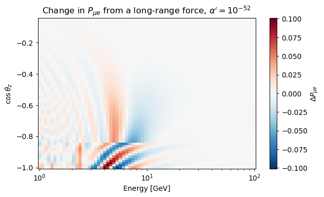
A long-range force from a gauged \(L_e - L_\mu\) symmetry, in energy and zenith angle. Code: notebook 20.

Between two places on the Earth

The chord between two named sites, and the probability along it. earth.probabilities_3nu_between_locations() does the lookup, the geometry and the PREM slabbing in one call.

for source, detector in (('cern', 'gran_sasso'),
                         ('fermilab', 'homestake'),
                         ('tokai', 'kamioka')):
    lat1, lon1 = earth.coordinates_of_named_location(source)
    lat2, lon2 = earth.coordinates_of_named_location(detector)
    chord = earth.chord_length_inside_earth(lat1, lon1, lat2, lon2)
    p_mue = earth.probabilities_3nu_between_locations(
        h_vacuum, 1.0*GEV, source, detector, n_slabs_per_segment=6)[3]
    print('%-22s %8.1f km   P_mue = %.6f'
          % (source + ' to ' + detector, chord, p_mue))

cern to gran_sasso        728.6 km   P_mue = 0.059820
fermilab to homestake    1284.7 km   P_mue = 0.020344
tokai to kamioka          294.7 km   P_mue = 0.033812

Those are the baselines the experiments quote: CNGS is 730 km, T2K 295 km. Fermilab to Homestake comes out at 1285 km against DUNE’s quoted 1300, the difference being that DUNE quotes the distance to the detector hall rather than the surface chord. Code: notebook 07.

An arbitrary matter profile

slabs takes any sequence of widths and Hamiltonians, so a profile can be built by hand. Castle-wall profiles are the interesting case: the arrangement of the matter can change the answer even when the mean density does not.

The effect is resonant, not generic — at most energies the two agree closely, and near a particular one they do not.

import slabs

widths_km = np.full(24, 250.0)
castle = np.where(np.arange(24) % 2 == 0, 2.0, 8.0)
uniform = np.full(24, castle.mean())

def appearance(densities, energy):
    h = hamiltonians3nu.hamiltonian_3nu_matter(
        h_vacuum, energy, earth.matter_potential(densities))
    return slabs.probabilities_3nu_slabs(h, widths_km*KM)[3]

print('mean density, both cases: %.1f g/cm^3' % castle.mean())
for energy_gev in (0.44, 3.0):
    print('E = %4.2f GeV : castle %.4f   uniform %.4f' %
          (energy_gev,
           appearance(castle, energy_gev*GEV),
           appearance(uniform, energy_gev*GEV)))

mean density, both cases: 5.0 g/cm^3
E = 0.44 GeV : castle 0.0104   uniform 0.0028
E = 3.00 GeV : castle 0.0457   uniform 0.0459

At 3 GeV the two are indistinguishable; at 0.44 GeV the castle wall gives nearly four times the appearance probability of a uniform slab of the same mean density.

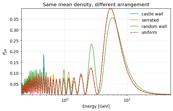
Four profiles, one mean density. Code: notebook 08.

Mass ordering and the octant

globaldefs carries the NuFit best fit for both orderings, so comparing them needs no numbers typed in. Matter is what separates them: the potential enters with a definite sign, so it enhances the resonance for one ordering and suppresses it for the other.

def h_vacuum_3nu(ordering='NO', s23=None):
    """Energy-independent vacuum Hamiltonian, for either ordering."""
    if ordering == 'NO':
        pars = (gd.S12_NO_BF, gd.S23_NO_BF, gd.S13_NO_BF,
                gd.DCP_NO_BF, gd.D21_NO_BF, gd.D31_NO_BF)
    else:
        pars = (gd.S12_IO_BF, gd.S23_IO_BF, gd.S13_IO_BF,
                gd.DCP_IO_BF, gd.D21_IO_BF, gd.D31_IO_BF)
    s12, s23_bf, s13, dcp, d21, d31 = pars
    return hamiltonians3nu.hamiltonian_3nu_vacuum_energy_independent(
        s12, s23_bf if s23 is None else s23, s13, dcp, d21, d31)


def p_matter(h, energy):
    """The nine probabilities in crust matter, at 1300 km."""
    return oscprob3nu.probabilities_3nu(
        hamiltonians3nu.hamiltonian_3nu_matter(
            h, energy, gd.VCC_EARTH_CRUST), 1300.0*KM)

print('normal   : Dm31 = %+.4e eV^2' % gd.D31_NO_BF)
print('inverted : Dm31 = %+.4e eV^2' % gd.D31_IO_BF)

for ordering in ('NO', 'IO'):
    print('  %s : P_mue at 2.5 GeV = %.4f'
          % (ordering, p_matter(h_vacuum_3nu(ordering), 2.5*GEV)[3]))

normal   : Dm31 = +2.5250e-03 eV^2
inverted : Dm31 = -2.4381e-03 eV^2
  NO : P_mue at 2.5 GeV = 0.0872
  IO : P_mue at 2.5 GeV = 0.0393

The octant of \(\theta_{23}\) is the other open question, and it needs the appearance channel rather than the disappearance one:

for s23_squared in (0.45, 0.55):
    p = p_matter(h_vacuum_3nu('NO', s23=np.sqrt(s23_squared)), 5.0*GEV)
    print('sin^2(theta23) = %.2f : P_mumu = %.4f   P_mue = %.4f'
          % (s23_squared, p[4], p[3]))

sin^2(theta23) = 0.45 : P_mumu = 0.4816   P_mue = 0.0245
sin^2(theta23) = 0.55 : P_mumu = 0.4768   P_mue = 0.0299

Disappearance depends on \(\theta_{23}\) mainly through \(\sin^2 2\theta_{23}\), which is symmetric about maximal mixing, so the two values either side of it are nearly indistinguishable there — the octant degeneracy. Appearance carries \(\sin^2\theta_{23}\) instead and tells them apart.

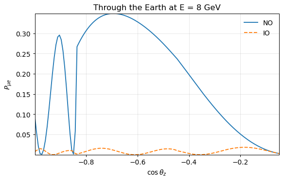
Matter through the Earth separates the two orderings. Code: notebook 12.

A sterile neutrino

Four flavors is the same call with a bigger matrix. A 3+1 scenario is a closed four-state system, not a leak out of the three-flavor block, which is what brings it inside an exact method at all.

import numpy as np

import globaldefs as gd
import hamiltonians4nu
import oscprob4nu

h4 = hamiltonians4nu.hamiltonian_4nu_vacuum_energy_independent(
    gd.S12_NO_BF, gd.S23_NO_BF, gd.S13_NO_BF,
    np.sqrt(0.10), np.sqrt(0.10), 0.0,
    gd.DCP_NO_BF, gd.D21_NO_BF, gd.D31_NO_BF, 1.0)

prob = oscprob4nu.probabilities_4nu(np.asarray(h4)/1.0e9,
                                    1300.0*gd.CONV_KM_TO_INV_EV)

print('%d probabilities, initial flavor slowest' % len(prob))
print('P(nu_mu -> nu_mu) = %.5f' % prob[5])
print('P(nu_mu -> nu_s)  = %.5f' % prob[7])

16 probabilities, initial flavor slowest
P(nu_mu -> nu_mu) = 0.40717
P(nu_mu -> nu_s)  = 0.01166

In matter the sterile state changes the problem qualitatively. It feels neither potential, so the neutral-current term — which is proportional to the identity across the three active flavors, and therefore invisible at two and three flavors — no longer cancels. Removing it from all four states costs only a global phase and leaves \(-V_{NC}\) on the sterile entry, and that entry is what places the sterile matter resonance.

h4_matter = hamiltonians4nu.hamiltonian_4nu_matter(
    h4, 1.0e9, gd.VCC_EARTH_CRUST, gd.VNC_EARTH_CRUST)

print('nu_e entry : %+.4e eV' % h4_matter[0][0].real)
print('sterile    : %+.4e eV' % h4_matter[3][3].real)

nu_e entry : +5.0149e-11 eV
sterile    : +4.0511e-10 eV

Through the Earth, the same PREM machinery applies: earth.probabilities_4nu_earth() cuts the chord at every shell boundary and builds both potentials per slab.

import earth

prob = earth.probabilities_4nu_earth(h4, 1.0e10, -0.8)
print('P(nu_mu -> nu_mu) through the Earth = %.5f' % prob[5])

P(nu_mu -> nu_mu) through the Earth = 0.73238

Full walk-through: notebook 16.

Where to go next

• Quickstart — the shortest path to a first probability.

• Methodology — what the SU(2), SU(3) and SU(4) expansions actually do, and the sign conventions that matter once a matter potential is added.

• API reference — the full API reference, generated from the docstrings.

• Notebook 17 — the same probabilities cross-checked against an independent external code, and against a published closed form, with the conventions that have to be matched first.

• Tutorial notebooks — twenty of them, carrying their figures inline, in reading order.