How the search works

This page introduces the vocabulary. Screening, striding, the arrival scan, scoring, closing, pruning — these words appear throughout the documentation, the code and the run summaries, and none of them is guessable from ordinary English. Read this before anything else that quotes a number.

The one question

Everything the tool does reduces to a single question, asked once per pixel of an elevation model:

From this patch of ground, is there a target surface at the right range, in the right direction, at the right relative orientation, with the right matter behind it?

That is what makes one engine serve two experiments that look nothing alike. GRAND wants terrain a few degrees below the horizon and tens of kilometres away, to catch radio from air showers started by Earth-skimming tau neutrinos. TAMBO wants a canyon wall two to five kilometres across, to catch the particles themselves. They differ in their numbers, not in their structure.

The seven stages

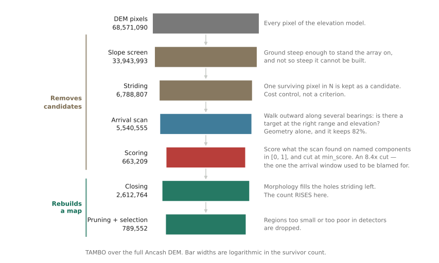
The figure is a real run — TAMBO over the full Ancash DEM, 68.6 million pixels — and the important thing about it is that it has two halves that work in opposite directions.

Everything down to scoring removes candidates. Everything below it rebuilds a map from what survived, which is why the count rises again at closing. Reading a funnel table as though every row were a filter is the commonest way to misread one.

The arrival scan and the scoring are two bars, and until recently they were one. The older funnel recorded the post-cut count under both names, so the merged bar read 1,022,530 and the arrival window carried the blame for a cut it had not made. Separated, the scan keeps 82% of what striding hands it and min_score takes 8.4× — the reverse of what a single bar implied, and the reason the stage is drawn on its own.

Stage by stage:

1. Screening. A cheap per-pixel test: slope inside the experiment’s deployable band, optionally altitude, aspect, distance to a road, and distance from a radio-noise zone. Slope is the one that matters — GRAND needs 3–25°, TAMBO 20–60°, and a pixel has only one slope, which is why co-location is decided here more than anywhere else.

2. Striding. Of the pixels that survive screening, one in candidate_stride is kept. This is cost control, not a criterion: the arrival scan is the expensive stage and its cost is linear in the number of candidates. Striding is unbiased in acceptance — measured identical at strides 1 and 5 — but it has a consequence at the far end of the pipeline that is easy to miss. See Striding and closing are one decision, not two.

3. The arrival scan. The heart of the tool. From each surviving candidate, walk outward along several bearings and, for each, find where the ray first meets terrain. A direction is accepted when that intersection lies in the configured distance window, the elevation window, and (optionally) strikes ground steep enough. One walk fills every elevation bin at once, so the azimuth count sets the cost and the elevation binning is nearly free.

4. Scoring. Each accepted candidate is given named component scores in [0, 1] — column depth, exit distance, accepted solid angle, shower development, tau decay, and others as configured — which are combined into one number and cut at min_score. See Why a product score has no safe threshold.

5. Closing. A morphological operation that fills holes. Its job is to undo striding: turn a lattice of isolated accepted marks back into a region a detector array could actually occupy.

6. Pruning and selection. Connected regions are labelled, then dropped if they are too narrow (min_width_km), too small, or hold too few detector positions (min_sub_array_size). What remains is the answer.

Striding and closing are one decision, not two

Subsampling is legitimate, and the reason is worth stating rather than asserting: a fraction survives sampling; a shape does not. Keeping one candidate in five tells you what share of the ground is viable to within a rounding error — 58.414% at stride 1 against 58.415% at stride 5 for GRAND, 75.750% against 75.736% for TAMBO. It does not tell you where, because a site is a place and not a statistic. So the map has to be rebuilt, and that rebuild is what closing is for.

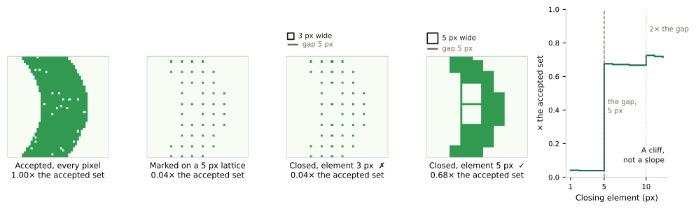
Striding leaves a gap of candidate_stride pixels between kept candidates. Closing repairs it — but only if its structuring element is larger than that gap. Below the gap the marks never touch and the mask stays a scatter of isolated pixels; above it the region reappears almost intact.

Closing is a dilation followed by an erosion. Dilation stamps the structuring element on every marked pixel; erosion then keeps only the ground where the whole element still fits. Gaps narrower than the element are filled, everything else returns to the shape it started as, and nothing is ever removed. Marks left on a lattice are therefore reconnected exactly when neighbouring stamps touch — which happens when the element is at least as wide as the gap. Below that the stamps stay apart, erosion peels each one back to the single pixel it grew from, and the output is identical to the input. That is why the comparison is a cliff and not a ramp: whether two stamps touch is a yes-or-no question.

The transition is at the gap and it is abrupt. In the figure a 3-pixel element recovers 0.04× of the accepted set and a 5-pixel one recovers 0.68× — seventeen times more, for two pixels of element. A second and far smaller step follows at twice the gap, where the element grows wide enough to bridge second-neighbour marks; it is worth 0.06× against the 0.64× at the gap.

One arithmetic note, because the figure and the pipeline stride differently. The figure thins a two-dimensional lattice, keeping every fifth row and column, so it marks one pixel in twenty-five. The pipeline thins the flat list of surviving candidates and keeps one in five — 3,853,258 to 770,652 for GRAND at Colca. Both leave the same five-pixel gap, which is the only thing the figure is about.

This is not a hypothetical. It is the mechanism behind a real 1.51× under-report of TAMBO’s area at Colca, and a 23.0× one on the steeper ground of the Callejón de Huaylas, where the accepted strips are narrower still. GRAND never suffers it: its 1 km closing element bridges a 154 m stride gap without noticing.

Both figures were far larger — 4.75× and 291× — when TAMBO’s element was 100 m rather than the published 150 m. Two extra pixels of element is the whole difference, which is the point of the arithmetic above rather than a footnote to it.

Warning

The damage is not done to the area measurement. It is done in pruning: a fragmented mask becomes thousands of tiny regions, and almost none of them clears min_sub_array_size. Every run warns when the element cannot bridge the gap (warn_stride_outruns_closing()). Heed it, raise ``gap_close_km``, or read the area as a lower bound and say so.

Why a product score has no safe threshold

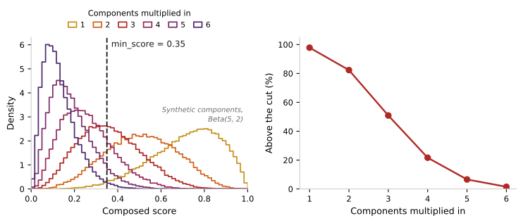
Components are combined by multiplication, so a candidate must be good at everything and one bad component sinks it. That is defensible — these are requirements, not preferences — but it has a consequence for any threshold placed on the result.

A product of several numbers in [0, 1] piles up near zero however good the terrain is. So min_score does not express a mild preference: it sits on a cliff, and where it lands depends on how many components happen to be enabled. Adding a component moves every score down and silently tightens the cut.

The figure above is a demonstration, not a measurement. Its six components are draws from a Beta(5, 2), deliberately generous — mean 0.714, mode 0.80 — so that the collapse cannot be blamed on poor terrain. What one real search does is a different and sharper story.

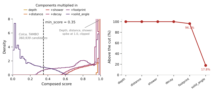
Every curve is the running product over the same 360,939 geometrically accepted candidates of one Colca TAMBO run, with one more component multiplied in. The population is fixed; no candidate is removed between curves and only the scores move.

depth and distance are exactly 1.0 for every candidate, and shower for 92.3% of them — so half the components do nothing whatever. Five of the six together still leave 96.3% above the shipped cut. The sixth, solid_angle, takes it to 17.8% and the median composed score to 0.13.

So the honest statement about min_score on this terrain is not that a product of six criteria has no natural threshold. It is that the cut is a cut on solid_angle, wearing a product as a disguise — the measured form of the caveat that solid_angle is the weakest component at every selected site in every region.

Measured on one real search, cuts of 0.0, 0.35 and 0.5 gave 65,268, 10,437 and zero detector positions. score_percentile is the scale-free alternative and is scored against the same ranking; see Assumptions and limitations.

Co-locating two arrays

The search answers where each experiment could go. Deployment asks something else: given a site chosen for one, is there enough ground nearby for the other?

The tempting way to ask is “how much of the joint region can host the partner”, and it is the wrong question even when it happens to give a workable answer.

At TAMBO’s old 100 m spacing it gave a spectacularly wrong one. The joint mask on the unbiased Cajatambo crop came to 22,577 fragments, of which exactly one was large enough for a single 1 km lattice cell, while roughly a thousand square kilometres of perfectly good GRAND ground lay within 20 km. An optimiser pointed at the intersection would have called that site impossible.

At the published 150 m the trap is much milder, and it is worth saying so rather than keeping the better story. The same crop now gives 91 fragments, of which 52 are large enough for that lattice cell, against 1,012.5 km² of GRAND ground within 20 km. A larger closing element stops shattering TAMBO’s mask, and the joint stops being confetti. The fragment count is the unambiguous part; how many fragments are “large enough” depends on what you demand of one, and 52 assumes a single hex cell at 1 km spacing.

The question is still the wrong one, though, and for a reason no spacing changes.

A partner array does not have to stand on the joint mask. What couples two arrays is a shared line of sight to the same massif, not a shared footprint, and GRAND’s own targets are 10–40 km away.

from oroscope import combine_experiments as ce

run = ce.load_run("output/ancash_full_grand")
ce.smallest_radius_for(run["mask"], run["world"], lat, lon, wanted=1000)

Measured from each region’s best TAMBO site, the answer is consistent:

Region	100 GRAND antennas	1,000	5,000
Arequipa	10 km	20 km	60 km
Ancash	10 km	30 km	60 km
Lima	10 km	30 km	60 km

None of the three is limited by finding partner ground near a site. The limit is simply that 1,000 antennas at 1 km spacing need 866 km², and steep country does not offer that within a few kilometres. Notebook 11 computes the table.

What the answer is, and is not

It is	It is not
A ranking of ground by how well it satisfies named geometric and physical criteria.	An event rate. No flux, no cross-section and no detector response are folded in. The scores are not apertures.
A capacity estimate for an arbitrarily placed array.	An optimised layout. Detectors are placed from each region’s bounding-box corner, not fitted — see Implementation notes.
Reproducible from a configuration file and a DEM.	Validated against an external simulation. Nothing here has been.

Assumptions and limitations is the blunt version of this table, and every run prints its own.

Where to go next

• Glossary — every term on this page, defined, with links to where it is used.

• Tutorial notebooks — notebook 7 animates the mechanisms above; notebook 8 drives the pipeline and reads its output; notebooks 9 to 12 are real regions.

• The physics — what the geometry gets multiplied by.

• Implementation notes — how it is actually built, for anyone changing it.