The physics
What the search is actually computing, why each criterion is there, and where each number came from. Assumptions and limitations states what is taken for granted and what that costs; this page is the derivation.
The question a site search must answer
Not “is there a tall mountain out there” but:
From this patch of ground, is there a target surface at the right range, in the right direction, at the right relative orientation, with the right matter behind it?
That phrasing is doing real work. It is what lets one engine serve experiments that look nothing alike. GRAND watches for radio from air showers started by Earth-skimming tau neutrinos, and wants terrain a few degrees below the horizon, tens of kilometres away. TAMBO watches for the particles themselves, across a canyon, two to five kilometres away. They differ in their numbers, not in their structure.
Tracing backwards from the detector
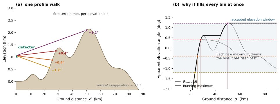
Fix a candidate pixel and an arrival direction: azimuth \(\phi\), elevation \(\theta\) measured from horizontal. Trace backwards along that direction.
Rays above the local horizon escape to the sky and meet no matter.
Rays below it strike terrain. That first intersection is where the tau left the rock, the distance to it is the decay baseline, and the path length beyond it that runs under the surface is the column depth.
Writing the elevation angle of the terrain at ground distance \(d\) as
a ray at angle \(\theta\) first meets terrain at the smallest \(d\) where \(\theta_{\rm terrain}(d) \ge \theta\). The \(d^2/2R\) term is the Earth’s curvature dropping distant ground away below a straight line.
One walk serves every elevation bin. Since the running maximum of \(\theta_{\rm terrain}\) only increases, each new maximum claims a contiguous band of elevation bins, so the first-intersection distances for all bins are filled in a single pass. Column depth follows from the same samples: the ray at angle \(\theta\) is underground wherever \(\theta_{\rm terrain}(d) > \theta\), so binning \(\theta_{\rm terrain}\) and taking an inclusive suffix sum gives the underground path length for every bin at once. Rays crossing several ridges accumulate all of the rock they traverse, not only the first chord.
This costs one profile walk per (candidate, azimuth) regardless of how finely the elevation window is sampled — which is why the elevation binning is nearly free and the azimuth count is what sets the cost.
Note
The walk works in slope, not angle. Every comparison it makes is monotonic in the elevation angle, so comparing \(\text{apparent}/d\) against pre-computed tangents of the bin edges gives identical decisions without an arctangent per sample.
A consequence that is easy to forget, and which has broken four separate tests in this project’s history: a detector standing on the ground has every steeply downward direction blocked by the ground at its own feet. A ray angled down more steeply than the slope it stands on intersects terrain within a pixel or two.
Two radii, because two different things propagate
Particles travel in straight lines. The neutrino and the tau are not refracted, so the geometry deciding where the tau exits uses the true Earth radius, 6371 km. That is not a modelling choice; it is what the trajectory is.
The radio signal is refracted by the tropospheric density gradient, and the standard \(k = 4/3\) convention makes a refracted ray straight again by inflating the radius to 8500 km. It applies to the Fresnel clearance of the signal path and to nothing else.
The difference is not negligible: over an 80 km path the apparent drop is 376 m at \(k = 4/3\) against 502 m at \(k = 1\), comparable to the Fresnel clearance itself.
The criteria, one at a time
Local terrain: slope and aspect
Slope is scale-dependent, and this is not a subtlety that can be ignored. On real Andean terrain the median slope falls from ~17.8° measured over the DEM’s native ~61 m to ~10.8° over 1 km, and the fraction passing a 3–25° band rises from 60% to 78%. Which of those is “the” slope depends on the footprint being deployed, so the measurement baseline is an explicit parameter rather than an accident of the DEM’s resolution.
import numpy as np
from oroscope import physics

# Slope enters the screen as a band on the squared gradient, which needs neither
# a square root nor an arctangent
from oroscope import site_searcher as ss
lo, hi = ss.slope_band_gradient_sq(3.0, 25.0)
print(f"3-25 deg is  {lo:.4f} <= dx^2+dy^2 <= {hi:.4f}")
3-25 deg is 0.0027 <= dx^2+dy^2 <= 0.2174
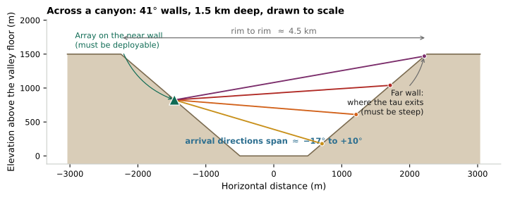
The band is per experiment, and probably per role. GRAND wants ground it can deploy on: 3–25°. Colca’s canyon walls are ~40°, far outside that. A single global slope band cannot express both, which is the clearest single argument for per-experiment criteria.
The slope band is not the only thing that differs. The two experiments ask the same structural question — is there a target surface, at the right range, in the right direction — at scales an order of magnitude apart, and one shared axis is the quickest way to see it.
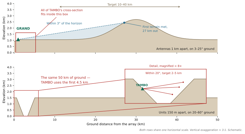
GRAND stands on ground inside its 3–25° band and watches a massif through a window 3° about the horizon; its sight line ends where it first meets ground, 27 km out here. TAMBO’s whole cross-section — the canyon drawn above, 4.5 km rim to rim — is the notch in the first tenth of the same axis, and it looks across 2–5 km through a window 20° wide.
Neither description conflicts with the other. They differ in range and in angle, not in kind, which is why one engine serves both and adding an experiment is a configuration rather than a code path. What the two genuinely compete for is the slope of the pixel they stand on — settled at the screening step, before any arrival geometry is considered.
The far wall
Slope at the candidate describes the near wall — the ground the array stands on. The far wall, which is where the tau exits, is a separate question, and asking only whether rock is present there is far too weak: on real Andean terrain something is nearly always present at some range and bearing. Before this criterion existed, 92% of candidates passed a canyon-shaped test.
The walk therefore records how fast the terrain was climbing along the ray where it was first met, \({\rm d}z/{\rm d}d\) between the previous sample and the intersection. Measured along the arrival azimuth, so an obliquely-viewed wall counts as the tau would actually cross it.
Column depth
The tau must be produced in the rock and must escape it, so column depth is a band, not a floor. Both edges are physical: too little rock and the neutrino does not interact; too much and the tau loses energy and decays before it reaches the surface.
The optimum runs from about 12 km of rock at 100 PeV to 23 km at 10 EeV — it is not flat with energy, which an early version of this code assumed.
Warning
Column depth is accumulated along the walk, and the walk stops at
max_dist_km. For a short-range search — TAMBO’s 5 km — the depth reported is
therefore bounded by how far is left to walk rather than by the far wall’s actual
thickness. See Assumptions and limitations.
Atmospheric depth, and why it differs by detection channel
A shower develops through grammage, not through metres, and air at 4000 m is a third thinner than at sea level. What “enough” means depends on what is being detected, and the two cases are genuinely different:
Radio. Emission comes from around shower maximum and then propagates through air that is effectively transparent at 50–200 MHz. Being far beyond maximum costs nothing directly, so the criterion is a threshold. The real trade at greater distance is amplitude against footprint area, which belongs to the footprint term.
Particles. The charged-particle content peaks at maximum and dies away after, so a particle array wants to sit near it and the criterion genuinely is a band.
The band follows from the primary energy through the shower profile:
from oroscope import physics

for e in (3.0, 55.0, 1000.0):
    print(f"{e:>7.0f} PeV:  X_max = {float(physics.shower_maximum_gcm2(e)):.0f} g/cm^2")

lo, hi = physics.grammage_band_from_energy(3.0, 1000.0, fraction=0.1)
print(f"\nTAMBO's 3 PeV - 1 EeV, at a tenth of peak content: {lo:.0f} - {hi:.0f} g/cm^2")
      3 PeV:  X_max = 561 g/cm^2
     55 PeV:  X_max = 631 g/cm^2
   1000 PeV:  X_max = 700 g/cm^2

TAMBO's 3 PeV - 1 EeV, at a tenth of peak content: 236 - 1287 g/cm^2
This matters for siting far more than it looks. A canyon crossing supplies only what its own width of air contains — about 170 g/cm² across 2 km of Colca and ~390 g/cm² across its full 4.5 km rim to rim. The default particle band of \((X_{\rm max}, 4X_{\rm max})\) = 700–2800 g/cm² rejects every canyon, which is how this was discovered.
Tau decay in the gap
The tau leaves the far surface and travels toward the detector; it is only useful if it decays with enough path left for a shower to develop. With \(L\) the boosted decay length,
import math
from oroscope import physics

for e in (3.0, 55.0, 100.0, 1000.0):
    L = physics.tau_decay_length_m(e)
    print(f"{e:>7.0f} PeV:  L = {L:>8.0f} m   P(decay within 3 km) = "
          f"{1 - math.exp(-3000 / L):.3f}")
      3 PeV:  L =      147 m   P(decay within 3 km) = 1.000
     55 PeV:  L =     2694 m   P(decay within 3 km) = 0.672
    100 PeV:  L =     4898 m   P(decay within 3 km) = 0.458
   1000 PeV:  L =    48980 m   P(decay within 3 km) = 0.059
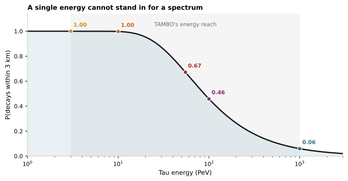
For GRAND this is largely implicit, because its distance window is derived from the decay length. For a canyon it is not: the window comes from the terrain, and across a 3 km crossing the probability runs from 1.00 at 3 PeV to 0.06 at 1 EeV. That is a factor of seventeen inside a single experiment’s energy reach, and it is invisible to every other term.
So the term is folded over the spectrum rather than evaluated at one energy. With a flux \({\rm d}N/{\rm d}E \propto E^{-\gamma}\),
That this matters is measurable rather than arguable. Sweeping the assumption each way:
Assumption swept |
Range |
Reported capacity |
|---|---|---|
single representative energy |
3 – 1000 PeV |
10878 → 0 |
spectral index, folded |
\(\gamma\) = 1.5 – 2.7 |
7205 → 10495 |
A single energy chooses the answer; folding makes it a property of the terrain and the
spectrum. The index itself may be pinned or left to vary: pass one value to state a
belief about the spectrum, or a (low, high) pair to marginalise uniformly over the
range, which is the honest form when the index is not known.
from oroscope import physics

pinned = physics.spectrum_weighted_decay_probability(3000.0, 3.0, 1000.0, 2.0)
spread = physics.spectrum_weighted_decay_probability(3000.0, 3.0, 1000.0, (1.5, 2.7))
print(f"gamma pinned at 2.0     : {float(pinned):.4f}")
print(f"gamma marginal 1.5-2.7  : {float(spread):.4f}")
gamma pinned at 2.0     : 0.9538
gamma marginal 1.5-2.7  : 0.9498
Geomagnetic emission
Radio emission goes as \(|\vec{v} \times \vec{B}|\): a shower travelling along the field radiates almost none of it. So the azimuth of a target matters, not merely its existence. At Arequipa this is worth a factor of 3.7 between east-facing and north-facing targets — larger than most of the geometric effects the search is weighing, and invisible to any purely geometric measure.
Irrelevant to a particle array, which is why it is switched off for TAMBO.
Fresnel clearance
The scan already guarantees nothing blocks the line of sight — the intersection is by construction the first terrain met — so this is a refinement rather than a gate: a ray that merely grazes a ridge suffers diffraction loss even though the geometric path is clear. The first Fresnel radius at distance \(d\) along a path of length \(D\) is \(r_1 = \sqrt{\lambda d (D-d)/D}\).
Two details that make the difference between a meaningful measure and a degenerate one. The far endpoint is the shower, not the exit point: taking the exit point makes both the clearance and \(r_1\) go to zero together, so the ratio collapses for every path regardless of what is actually in the way. And the antenna sits at a stated height above ground, because a receiver at ground level always has terrain inside its own first Fresnel zone.
Earth absorption
For downgoing directions the neutrino has crossed a chord of the Earth, \(2R \sin\theta\), which dwarfs local topography. The suppression narrows the effective arrival window with energy: its lower edge climbs from −4.4° at 100 PeV to −0.9° at 10 EeV.
That is a falsifiable prediction, and worth checking against a collaboration’s own simulated acceptance. If their window does not narrow that way, one of the two treatments has the absorption wrong.
Two signals, two physics
Everything above is common machinery: one profile walk, one geometric question. What makes GRAND and TAMBO different is not the terrain analysis but what reaches the detector, and almost every difference in their configurations follows from that one fact. It is worth separating them properly, because the criteria that look arbitrary side by side are each forced by the signal.
GRAND: radio from the air shower
The tau exits the rock, decays, and the resulting air shower radiates coherently at tens to hundreds of MHz. The detector never sees a particle. It sees an electromagnetic pulse, and that changes what the terrain has to provide.
The air must be transparent, and it is. Radio at 50–200 MHz propagates essentially unattenuated through the atmosphere. Emission comes from the region around shower maximum and then simply travels. So the grammage criterion is a threshold — the shower must have reached maximum — and not a band. Being far past maximum costs nothing directly.
The signal path must be clear. Because it is a wave, an obstruction inside the first Fresnel zone diffracts it. This is why GRAND alone carries a Fresnel clearance criterion, an antenna height, and a near-field exclusion, and why it needs the \(k = 4/3\) radius: the radio ray bends and the particle trajectory does not.
The emission is anisotropic, and the anisotropy is geomagnetic. The dominant mechanism is transverse current driven by the geomagnetic field, so the amplitude scales with \(\sin\alpha\), the angle between the shower axis and \(\vec{B}\). At Arequipa’s field this is not a detail: an east-facing target is worth 3.7× a north-facing one. A criterion that ignored it would rank sites by geometry alone and get the ordering wrong.
The footprint sets the spacing. The Cherenkov cone is about a degree, and its radius on the ground grows with distance and shrinks with altitude — thinner air means smaller \(n - 1\), a narrower cone, a smaller footprint, and so a denser array for the same trigger efficiency. Hence 1 km spacing, tens of thousands of antennas, and a deployable band of 3–25°: an antenna array is a compact blob on open ground, not a strip.
Which fixes the range. 10–40 km: far enough that the shower has developed and the footprint is large, close enough that the signal survives and the geometry stays within a few degrees of the horizon.
TAMBO: the particles themselves
TAMBO puts water-Cherenkov tanks on a canyon wall and waits for the shower to arrive as matter. Every difference follows.
The shower must be alive when it arrives. Charged-particle content peaks at shower
maximum and then dies away, so grammage is a band, not a threshold — too little air
and the shower has not developed, too much and there is nothing left to detect. This is
the single most consequential difference from GRAND, and it is why
grammage_mode: "particle" exists as a separate mode rather than a tuned threshold.
Nothing propagates as a wave, so several criteria simply switch off. No Fresnel clearance, no antenna height, no geomagnetic weighting — the particles do not care about \(\vec{B}\), and a criterion left switched on here would be weighting by a mechanism that is not operating.
The target is the opposite wall, not the horizon. 2–5 km rim to rim, roughly 1.5 km deep. That short baseline is what makes the tau decay length so decisive: at 1 EeV the decay length is ~49 km against a ~3 km crossing, so only a few per cent of taus decay in time. This is the criterion that most rewards folding over the spectrum rather than picking an energy — the same search gave 10 878 detector positions at 3 PeV and zero at 100 PeV.
The geometry is two-sided. One wall is where the array stands (20–60°) and the other is where the tau exits (≥25°, measured along the arrival azimuth at the point the ray strikes). Without the second, the scan only asks that rock is present at the right range, which is true almost everywhere in the Andes.
And the array is a strip. 150 m spacing along a wall, so min_width_km must be 0 —
the opening step that prunes tendrils would otherwise delete exactly the shape TAMBO
is. Looking across a canyon also accepts far more sky than looking to the horizon: 0.2–
0.5 sr against GRAND’s ~0.017, which is why the solid-angle half-value has to be
experiment-specific or the term saturates and stops discriminating.
What each signal tells you about the shower
The two channels do not measure the same quantity less or more well. They measure different things, and that is the whole argument for a joint site.
Radio measures the electromagnetic shower, calorimetrically. The field amplitude scales with the energy in the electromagnetic cascade, and the atmosphere neither absorbs nor scatters at these frequencies — so what arrives at the antenna is what was emitted, with no attenuation correction to make and no dependence on how much shower happens to survive to the ground.
Three further things come with it, and none has a particle-array equivalent:
The direction, from the arrival times of a nanosecond pulse across the array.
The depth of shower maximum, from the shape of the arriving wavefront and the slope of the lateral distribution. \(X_{\rm max}\) is the classic handle on how deep the shower developed — and for a tau shower it constrains where the decay happened, which is the geometry this whole search is about.
The polarisation, which identifies the emission mechanism: geomagnetic emission is polarised along \(\vec{v} \times \vec{B}\) and charge-excess emission radially about the axis. That is a physical signature no anthropogenic pulse reproduces, and it is the main defence against the radio-frequency interference the RFI criterion otherwise has to exclude geometrically.
What radio does not give is the particle content. It is nearly blind to muons, which carry little of the electromagnetic energy.
Particles measure the shower where it is, at one depth. A water-Cherenkov array counts what physically arrives: the density and arrival times of particles at the ground. That is a sample of the longitudinal profile at a single slice — the ground — which is why TAMBO’s grammage criterion is a band. Miss the slice and there is nothing to detect.
In exchange it sees what radio cannot:
The muon content. Muons penetrate where the electromagnetic component is absorbed, and a water-Cherenkov tank distinguishes them by the depth of light they deposit. Muon number is the standard discriminator of shower composition, and it separates a hadronic cascade from a purely electromagnetic one.
A direct count, with no emission geometry in the way. There is no Cherenkov cone to sit inside and no magnetic-field angle to be unlucky in: if the particles arrive, they are detected.
Both together give what neither gives alone. Three things, in increasing order of what they are worth:
Two points on one longitudinal profile. Radio gives \(X_{\rm max}\), where the shower peaked; the array gives its content at the ground. Two depths on the same cascade constrain the shower age — and therefore the altitude and distance at which the tau decayed — far better than either does alone.
Energy and composition separately. Radio measures the electromagnetic energy calorimetrically and the array measures the muon number. Those are the two numbers a shower measurement wants, and each channel supplies the one the other is blind to. For a tau shower they also begin to separate the decay channel, since a hadronic decay produces muons that an electromagnetic one does not.
Cross-calibration on the same event, which is the real prize. Radio’s systematics are the antenna response, the electronics and the emission model. The array’s are the tank response and the hadronic interaction model. These are almost entirely independent, so a shower measured by both constrains each in a way that neither can constrain itself. Every energy scale in this field is limited by exactly that kind of systematic, and coincident events are how it is attacked.
There is a fourth, less glamorous and possibly more immediately useful: a coincidence is essentially unfakeable. A radio pulse with the right polarisation arriving at the same instant as particles on the ground is not something a power line, an aircraft or a mine does.
Side by side
GRAND (radio) |
TAMBO (particle) |
|
|---|---|---|
What arrives |
a coherent radio pulse |
the charged particles |
Grammage criterion |
threshold — the air is transparent |
band — the shower dies after maximum |
Fresnel clearance |
required |
not applicable |
Geomagnetic weighting |
dominant, 3.7× east over north |
off |
Earth radius used |
\(k=4/3\), 8500 km, for the signal |
true, 6371 km |
Target range |
10–40 km, to the horizon |
2–5 km, across a canyon |
Deployable slope |
3–25° |
20–60° near wall, ≥25° far wall |
Array shape |
compact blob, 1 km spacing |
strip, 150 m spacing |
Accepted solid angle |
~0.017 sr |
0.07–0.5 sr |
What it measures |
EM energy, calorimetrically; \(X_{\rm max}\); polarisation |
particle density at the ground; muon content |
Blind to |
muons |
the shower above the ground |
Design reference |
[Arguelles+26], [RW+20] |
Joint particle + radio arrays
The interesting question is not whether either experiment can be sited, but whether one patch of ground can host both. That is a different question from either search, and it is easy to answer wrongly.
What a joint site actually is
A joint site is ground that satisfies both experiments’ demands on the ground itself. The distinction that matters:
Properties of the ground are shared. A pixel has one slope, one altitude, one aspect. If GRAND needs 3–25° and TAMBO needs 20–60°, both must accept that single number, and only the 20–25° sliver can. That sliver is 23% of the narrower band, and it is what decides co-location at Colca.
Properties of the view are not shared. What each experiment asks of the sky — the distance window, the arrival elevations, the far-wall slope — constrains a direction, not the ground. Two experiments can stand on the same hillside and look out at completely different ranges without conflicting: GRAND looking 10–40 km to the horizon and TAMBO looking 2–5 km across a canyon are not competing for anything.
Warning
This distinction is not academic, and getting it backwards produces a confident wrong answer. An early version of the combination summary reasoned about the viewing windows as though they were shared constraints, concluded that GRAND and TAMBO “cannot share ground at all”, and printed that directly above the ground they demonstrably share — 50 km² as measured then, 619.1 km² as measured now. A summary that reasons can be wrong in ways one that merely restates cannot, and it will be wrong persuasively.
What was measured
Over the full Arequipa DEM — 128.6 Mpx, a 117,430 km² footprint:
area km² |
of its own ground in the joint |
detectors |
|
|---|---|---|---|
GRAND alone |
88,208.2 |
0.7% |
101,584 |
TAMBO alone |
1,036.9 |
59.7% |
49,271 |
joint |
619.1 |
||
union |
88,626.0 |
The asymmetry is the whole story: essentially all of the joint is TAMBO’s ground, and a rounding error of GRAND’s. GRAND has so much deployable terrain that co-location costs it nothing; TAMBO has so little that three fifths of what it has is shared.
The claim that used to stand here — that the joint barely moved with scale — did not survive the re-run, and it is worth saying why rather than quietly restating it. At TAMBO’s old 100 m spacing the Colca crop gave 50.1 km² of joint and the whole DEM 50.2, which read as searching twenty-one times more ground found no additional co-locatable ground. At the published 150 m the crop gives 123.3 km² and the DEM 619.1, five times as much. The opportunity is not confined to Colca after all; the rest of the region’s canyons do offer it, and the old conclusion was an artefact of an element too small to reconnect what striding had cut apart.
One caveat holds in both versions and was never stated: the crop is measured at
downsample_factor 1 and the department at 4, so the two areas are not taken on the
same grid. The comparison is indicative of scale, not a like-for-like ratio.
Why one would want it
Three reasons, in increasing order of scientific interest.
Shared infrastructure. One site, one road, one power feed, one permit. For an observatory in a canyon at 4000 m this is not a minor line item.
Complementary energy coverage. TAMBO reaches roughly 3 PeV–1 EeV and GRAND above ~100 PeV. A joint site spans both with one deployment, and the overlap region is where the two are directly comparable.
Cross-calibration, which is the real prize. The same air shower seen simultaneously as a radio pulse and as particles on the ground is the cleanest possible handle on the energy scale of both techniques. Radio calorimetry and particle counting have almost entirely independent systematics; a shower measured by both constrains each in a way neither can constrain itself. That is an argument for co-location that survives even if the shared-infrastructure saving turns out to be small.
How to read the joint number
Every caveat on the individual runs applies here and compounds.
Both masks have already been morphologically closed, so the joint is the intersection of two inflated masks and is inflated twice over.
TAMBO’s area is a lower bound by 1.51× — measured with a stride-1 control at its own element size. It was 4.75× at the old 100 m spacing. Since the joint is almost entirely TAMBO’s ground, the joint is a floor too.
The overlay itself is exact: the masks are pixel-aligned and the alignment is checked rather than assumed. What it overlays is only as good as each run.
Co-location is a question about ground, not detectors. Two experiments sharing a hillside still need their own arrays, spacing and trigger. What they share is the site.
Scoring
Each criterion becomes a component in \([0, 1]\) — a band, a saturating function, or a ramp — and the components are composed. Storing the distributions rather than a single number is deliberate: absolute apertures can then be obtained later by folding against an acceptance table, without re-running the terrain analysis.
Warning
The default composition is a product of six components. A product of six numbers
in \([0,1]\) concentrates near zero, so a score threshold anywhere in the middle
sits on a cliff — measured, a TAMBO search returns 45 928 detector positions at
min_score 0.0, 2056 at 0.35, and zero at 0.5. Ranking sites and taking the best
\(N\) is better behaved than thresholding a product. See Assumptions and limitations.
From accepted pixels to a site
Three steps, each of which changes the answer and none of which is pure physics.
Morphological closing fills gaps between accepted pixels so that a site is a
deployable region rather than a scatter. It also inflates: measured with a stride-1
control run at Colca, closing with a 1 km element more than doubles the accepted area
(2.35×). The reported area is not the physics-accepted area, and the gap is now a
parameter, gap_close_km, rather than being tied to the detector spacing.
Warning
The closing element must outrun the gap that striding leaves. candidate_stride
marks one accepted pixel in \(N\); at Colca’s 30.7 m pixels, stride 5 leaves gaps
of 154 m. GRAND’s 1 km element bridges those easily. TAMBO’s element is
antenna_spacing_km = 100 m, which does not, so its mask never reconnects: it
stays a scatter of isolated pixels, most regions fall below min_sub_array_size,
and the area collapses.
Measured with a stride-1 control at TAMBO’s own settings: acceptance is unbiased (75.736% against 75.750%) while the reported area is 1.51× too small — 203.0 km² against 307.2. Striding is fair about which pixels it tests and destructive about which survive to be measured. Every run now warns when the element cannot bridge the gap. At the old 100 m element the same penalty was 4.75×, and the acceptance pair read 17.49% because the funnel then counted geometry and the score cut as one stage.
Opening prunes tendrils narrower than min_width_km. This encodes a GRAND
assumption — that an array is a compact blob — and it deletes exactly the long thin
strip that a canyon-wall array is. Set it to 0 for strip layouts.
Capacity places detectors in continuous ground coordinates on a square or triangular lattice and counts those landing on usable ground. Positions are laid out in metres and only then looked up in the pixel grid; converting the spacing to an integer pixel stride, as an earlier version did, truncates and packs detectors closer than asked — 7.4% high at 1 km spacing and 58% at 100 m.
import numpy as np
from oroscope import site_searcher as ss

# 3 km x 3 km of usable ground, 30 m pixels, 1 km triangular spacing
mask = np.ones((100, 100), dtype=bool)
n = ss.count_grid_capacity(mask, 30.0, 30.0, 1000.0, 1)
area_km2 = (100 * 30 / 1000.0) ** 2
analytic = area_km2 / (np.sqrt(3) / 2 * 1.0 ** 2)
print(f"{n} detectors on {area_km2:.1f} km^2; analytic density gives {analytic:.1f}")
12 detectors on 9.0 km^2; analytic density gives 10.4
The papers behind these numbers are collected on the References page.