Adiabatic + Magnus Hybrid Strategy

This page documents the strategy parameter accepted by magnus.oscprob.osc_prob_matter_std_potential(), magnus.oscprob.osc_prob_matter_nsi(), magnus.oscprob.osc_prob_liv(), and every wrapper built on them (every osc_prob_*_sun, osc_prob_*_sun_nsi, and osc_prob_*_sun_liv function, and every osc_prob_*_matter_exp_density function), as well as the fully generic, arbitrary-Hamiltonian entry points magnus.oscprob.osc_prob_sun() and magnus.oscprob.osc_prob_earth(): what problem it solves, the numerical method behind it (magnus.adiabatic), and the evidence used to validate it. See What “accurate” means here and Methodology for the plain Magnus-expansion machinery this strategy sits alongside.

The problem: extreme accumulated phase

The plain Magnus engine (Methodology) partitions a trajectory into slabs and is exact, to any desired order, within each one – but it must still resolve however many radians of phase accumulate inside a slab. For an \(\rm MeV\)-scale solar neutrino crossing most of the Sun’s radius, the vacuum term alone (\(\Delta m^2/2E\), growing as \(1/E\)) accumulates \(\mathcal{O}(10^3\text{--}10^6)\) radians. Reaching a requested tolerance then requires a very large number of slabs; if a refinement cap is hit first, osc_prob returns its best estimate but raises ToleranceNotAchievedWarning – correctly signaling that the result may be inaccurate, but not, by itself, a solution.

Physically, however, nothing is actually happening quickly here: away from a level crossing, the flavor content evolves adiabatically, tracking the instantaneous eigenstates of the Hamiltonian smoothly as the matter potential falls off. This is precisely the regime the Mikheyev-Smirnov-Wolfenstein (MSW) effect describes for solar neutrinos [GK07]: away from the resonance, the evolution is adiabatic and computable from the instantaneous eigenbasis alone, with no need to resolve the fast oscillation phase at all. The hybrid strategy in magnus.adiabatic automates exactly this: use adiabatic transport where it is valid, and reserve an exact (Magnus) computation for the narrow region, if any, where it is not.

Adiabatic transport

Let \(H(l)\) be diagonalized at each position, \(H(l) = W(l)\, \mathrm{diag}(\lambda_1(l), \ldots, \lambda_d(l))\, W(l)^\dagger\). The adiabatic theorem says that, as long as no two eigenvalues become (nearly) degenerate along the trajectory, a state that starts as the \(k\)-th eigenstate stays the \(k\)-th eigenstate, up to a phase:

\[|\psi_k(l)\rangle \approx e^{-i\Phi_k(l)}\, e^{i\gamma_k(l)}\, |v_k(l)\rangle , \qquad \Phi_k(l) = \int_{l_0}^{l} \lambda_k(s)\, ds ,\]

with \(\Phi_k\) the ordinary dynamical phase and \(\gamma_k\) the geometric (Berry) phase, generated by how the eigenvector itself turns as \(l\) varies. Assembled into an evolution operator in the original (flavor) basis, this is

\[U_{\rm adiabatic}(l_1, l_0) = W(l_1)\, \mathrm{diag}\!\left(e^{-i\Phi_k(l_1)}\right)\, W(l_0)^\dagger .\]

magnus.adiabatic.adiabatic_propagator() computes exactly this, integrating \(\Phi_k\) with Simpson’s rule over a grid of diagonalized Hamiltonians. It never has to resolve the accumulated phase step by step the way a Magnus slab or an ODE solver does – \(\Phi_k\) is a smooth, slowly-varying integral regardless of how large it eventually gets – so its cost is essentially independent of how many e-folds of the density profile the trajectory spans. The geometric phase needs no separate formula: at each grid step, \(W\)’s columns are phase-fixed by maximizing the (real, positive) overlap with the previous step’s eigenvectors – a discrete realization of parallel transport that captures \(\gamma_k\) implicitly, for genuinely complex Hamiltonians (nonzero CP-violating phases) exactly as well as real ones. The result is exactly unitary by construction (a diagonal phase conjugated by unitary matrices), independent of how fine the grid is; grid density only controls how well the discretized integral and parallel transport approximate the continuum adiabatic limit.

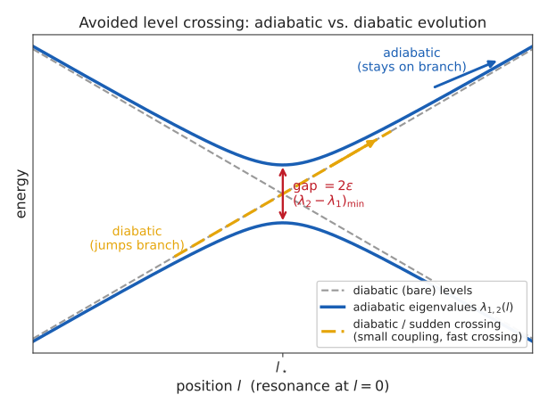
Two levels approach each other as a function of position \(l\) and avoid crossing, with minimum gap \(2\varepsilon\) at \(l_\star\). An adiabatic trajectory (blue) stays on its eigenvalue branch through the crossing; a diabatic trajectory (gold) instead follows the original (bare, dashed) levels straight through – the sudden, non-adiabatic transition the local Magnus patch exists to capture.

Detecting resonances without differentiating eigenvectors

Adiabatic transport breaks down where two eigenvalues nearly cross: the gap in the denominator above becomes small, and the state can no longer “keep up” with how fast the instantaneous eigenbasis rotates. Locating these points, and quantifying how badly adiabaticity is violated there, needs the derivative of the eigenvalues and eigenvectors along the trajectory – but eigenvectors are only defined up to a phase (and, at a near-degeneracy, up to an arbitrary rotation within the near-degenerate subspace), so differentiating them directly by finite differences is numerically fragile. The Hellmann-Feynman theorem avoids this entirely: for a normalized eigenvector \(|v_k(l)\rangle\) of \(H(l)\),

\[\frac{d\lambda_k}{dl} = \left\langle v_k(l) \right| \frac{dH}{dl} \left| v_k(l) \right\rangle , \qquad \left\langle v_j(l) \right| \frac{dH}{dl} \left| v_k(l) \right\rangle = (\lambda_k - \lambda_j)\left\langle v_j \left| \frac{dv_k}{dl} \right.\right\rangle \ \ (j\neq k) ,\]

exact identities that need only \(dH/dl\) – an ordinary derivative of the (smooth, gauge-independent) Hamiltonian itself, not of its eigenvectors. magnus.adiabatic.find_resonance_candidates() uses the first identity to locate every position where some pair of levels’ gap is stationary (\(d(\lambda_j-\lambda_k)/dl = 0\), an exact critical point, refined to machine precision by bisection), scanning every pair \((j,k)\), for a Hamiltonian of any dimension. Because every pair is scanned, no number of simultaneous resonances defeats the search: a crossing between one pair is never masked by a window belonging to another (verified at 2, 3, 4 and 5 flavors against a dense per-pair \(\gamma\) scan). What bounds the search is instead the probe grid: candidates are bracketed on n_probe linear samples, so a feature much narrower than \((l_1-l_0)/n_\text{probe}\) can be stepped over entirely and reported as no resonance at all. Supply t_breakpoints at a known narrow feature, or raise n_probe. The second identity then gives an exact, gauge-independent adiabaticity parameter, the Landau-Zener-like

\[\gamma_{jk}(l) = \frac{\left|\left\langle v_j(l)\right| dH/dl \left|v_k(l)\right\rangle\right|}{\left(\lambda_k(l) - \lambda_j(l)\right)^2} ,\]

with \(\gamma_{jk} \gg 1\) signaling a genuinely non-adiabatic (sharp/diabatic) crossing and \(\gamma_{jk} \ll 1\) a safely adiabatic one. Both quantities are evaluated from \(H(l)\) and its eigendecomposition alone, so they apply identically to a hand-built toy Hamiltonian, a real 3-flavor standard-oscillation Hamiltonian, or a 5-flavor (3+2 sterile) Hamiltonian with NSI and LIV terms – nothing about the detector assumes any particular structure.

Important

\(dH/dl\) is computed with an ordinary real finite difference, not complex-step differentiation (\(\mathrm{Im}[H(l+ih)]/h\)). Complex-step differentiation is only valid for functions that are real-valued at real input; \(H(l)\) here is routinely complex-valued even at real \(l\) (any nonzero CP-violating phase), and applying complex-step differentiation to it divides an \(l\)-independent complex Hamiltonian entry by the (tiny) differentiation step, producing derivatives wrong by many orders of magnitude. This was an early implementation bug, caught by comparing against a real-valued toy Hamiltonian (where the same complex-step formula happened to work by coincidence, since the function actually was real-valued there) – a cautionary example of why this module never uses it, on any Hamiltonian, real or complex.

Growing and merging non-adiabatic windows

A candidate with \(\gamma_{jk}\) above a threshold marks a position that needs an exact patch, but not, by itself, a window: the region over which adiabaticity is violated has a physical width that has nothing to do with the arbitrary spacing of the search grid used to locate the candidate in the first place. magnus.adiabatic() grows a window outward from each candidate by doubling the step size until \(\gamma_{jk}\) drops back below threshold, then pads it by a safety factor – a physical width, not a search-grid artifact (verified directly: the same physical case gives the same window regardless of how fine or coarse the initial search grid was). Windows from different candidates that end up overlapping or touching are merged into one, so that two resonances close enough together (or a resonance revisited from the “other side” by level repulsion near another crossing) are patched as a single contiguous region rather than double-counted, under-patched, or silently dropped.

Patching, and composing the pieces exactly

Inside a non-adiabatic window \([l_b, l_c]\), adiabatic transport is simply not trusted; instead, the package’s own Magnus kernel (magnus.magnus.magnus_expansion_multislab()) computes the evolution operator there directly, doubling the number of slabs until two successive levels agree. Since \([l_b, l_c]\) is narrow by construction (that is exactly what “window” means here), this exact computation is cheap even though the plain Magnus method would be slow over the whole trajectory.

The full hybrid propagator over \([l_0, l_1]\) with windows \([l_b^{(1)}, l_c^{(1)}], \ldots, [l_b^{(n)}, l_c^{(n)}]\) is then assembled by the exact composition law of quantum evolution,

\[U(l_1, l_0) = U_{\rm ad}(l_1, l_c^{(n)}) \cdots U_{\rm patch}(l_c^{(1)}, l_b^{(1)})\, U_{\rm ad}(l_b^{(1)}, l_0) ,\]

which holds regardless of which method computed each factor – the same principle the plain Magnus engine already relies on to chain ordinary slabs (Methodology). Every factor here (\(U_{\rm ad}\) from adiabatic_propagator(), \(U_{\rm patch}\) from the Magnus kernel) is exactly unitary by construction, so the composed \(U\) is exactly unitary too, regardless of how accurate the adiabatic approximation actually is anywhere along the way.

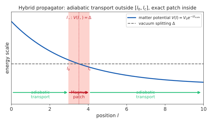
The hybrid propagator’s segmentation along a trajectory with one resonance: adiabatic transport everywhere except the narrow window \([l_b, l_c]\) bracketing the crossing \(l_\star\), patched with an exact local Magnus computation.

Self-certification

None of the tolerances above – the adiabaticity threshold, the density of the grid used to integrate the dynamical phase, or the density of the probe grid used to locate candidates – has a single value that is safe for an arbitrary Hamiltonian. A fixed threshold that is comfortably conservative for one case can under-patch another (this was checked directly during development: a fixed threshold=0.1 gave a 2% error on one engineered case, needing 0.01 for better than \(10^{-4}\)). magnus.adiabatic.hybrid_propagator() therefore never trusts a single evaluation: it repeats the entire computation with the threshold tightened (divided by 3) and the two grid densities doubled, together, comparing successive results, and only reports the result as certified once two successive levels agree within the requested rtol/atol – the same successive-refinement discipline magnus.oscprob.osc_prob() already uses for its own slab count. If a local patch itself fails to converge within its own slab cap, or the refinement loop exhausts its iteration budget without two levels agreeing, the propagator returns its best estimate (still exactly unitary) but reports it as not certified.

The strategy parameter

osc_prob_matter_std_potential, osc_prob_matter_nsi, and osc_prob_liv (and, transitively, every wrapper built on them), as well as osc_prob_sun and osc_prob_earth (via _osc_prob_with_potential, for a fully arbitrary user-supplied Hamiltonian), accept a strategy keyword, checked in this order for every requested (energy, baseline) point:

'magnus'

Use only the traditional Magnus-expansion machinery: the closed-form two-flavor interaction-picture integrator when it applies (still restricted to genuinely two-level Hamiltonians and a tagged exponential profile – see Methodology), the energy-batched scan engine, or the general adaptive slab-refinement method. This reproduces the exact behavior of Magνs as it was before the adiabatic strategy was added, unconditionally. It therefore opts out of the cumulative baseline scan as well, which postdates that behavior and builds a different slab grid: strategy='magnus' is the way to reproduce older numbers exactly, on a baseline scan as much as at a single point.

'hybrid'

Additionally try magnus.adiabatic.hybrid_propagator() for any point where the matter potential is position-dependent and no t_slab_edges/breakpoints were supplied (a piecewise-discontinuous profile such as PREM breaks the finite-difference diagnostics this method relies on) and a target tolerance was requested (the method is fundamentally adaptive; it has no “run once, fixed” mode). If the result fails to self-certify for at least one requested point, the best-effort result is still returned, together with HybridCertificationWarning (a subclass of ToleranceNotAchievedWarning, so existing code filtering on the parent class also catches it).

'auto' (default)

Try 'hybrid' first, under the same conditions, but fall back silently to the 'magnus' strategies above – no warning about the hybrid attempt itself – for any point where it does not apply or fails to self-certify.

It also stands aside for a baseline scan at a single energy with at least HYBRID_YIELDS_TO_CUMULATIVE_MIN_POINTS points. The hybrid strategy handles such a scan one point at a time, whereas the cumulative scan (see the cumulative parameter of magnus.oscprob.osc_prob_energy_baseline()) answers every baseline from a single traversal: measured on solar profiles, tens of times faster at equal or better accuracy. Below that number of points the hybrid strategy is the cheaper of the two and keeps the scan.

Unlike the two-flavor interaction-picture fast path, the hybrid strategy has no restriction on the number of flavors: the resonance detector and adiabatic propagator make no assumption about the Hamiltonian’s dimension or structure. It composes correctly with any number of simultaneous or sequential resonances, of any kind (standard MSW, NSI-induced, or otherwise), between any pair of levels, provided each is visible on the probe grid – see the two limits below.

Warning

Two things this strategy cannot see, both of which make it return certified=False or, in the second case, a wrong answer:

• A profile that is not smooth at the probe scale. Every diagnostic here finite-differences \(H(l)\) between probe points. On a density step, a kink, or any feature sharp compared with the probe spacing, those derivatives are meaningless. hybrid_propagator now measures this directly (magnus.adiabatic._profile_is_resolved) and declines to certify, so magnus.oscprob.osc_prob() falls through to the general Magnus path, which handles such profiles correctly. Passing t_breakpoints at the discontinuities is better still.

• A feature narrower than the probe spacing, which no fixed grid can detect: neither the probe nor its refinement samples it, so \(\gamma\) looks small and no window opens. Measured on a Gaussian resonance of width \(10^{-5}(l_1-l_0)\), the returned probability was wrong by 2.9e-02 while reporting certified=True. The general Magnus path is no better here (it misses the feature too, though it does warn). If a narrow feature’s position is known, pass t_breakpoints.

Note

That last sentence was, until version 1.0.0, true only of resonances that sit at an extremum of the level gap. The detector locates candidates as gap extrema and evaluated the adiabaticity parameter \(\gamma\) only there – but a gap extremum is where the gap is stationary, which is not where \(\gamma = |\langle v_j|\,dH/dl\,|v_k\rangle| / (\lambda_k - \lambda_j)^2\) peaks. On a rapidly varying profile the two differ sharply: measured on a solar exponential modulated by a strong sine with an NSI coupling, \(\gamma\) reached 3.6e-04 at the extrema against 7.0e-02 along the path, a factor of 196.

The consequence was worse than a loose estimate. No window opened, so successive refinements differed only in the adiabatic-transport grid, converged to the same wrong adiabatic limit, agreed with each other, and the result was reported as certified while being wrong by 4.3e-02 against solve_ivp. magnus.adiabatic.find_nonadiabatic_windows() now also sweeps \(\gamma\) along the probe grid, opening one window per contiguous stretch that exceeds the threshold, which brings that case to 2.2e-04 and leaves well-behaved profiles bit-for-bit unchanged.

import magnus.oscprob as oscprob
import magnus.globaldefs as gd

# 8 MeV, 90% of the way through the Sun: deep in the regime that used to
# need a very large slab count (and could hit ToleranceNotAchievedWarning)
# under strategy='magnus'.
P = oscprob.osc_prob_3nu_sun(
    8.0 * gd.UNIT_MEV, 0.9 * gd.SUN_RADIUS * gd.UNIT_KM, 0.0,
    strategy='auto',  # the default; shown explicitly here for clarity
)

Validation

Every claim above is checked directly against a tight-tolerance scipy.integrate.solve_ivp (DOP853) solution of the same Schrödinger equation, across a validation grid designed to exercise every qualitatively different case: zero resonances (purely adiabatic), one resonance, two well-separated resonances, and two resonances close enough together that their windows must merge; real 3-, 4-, and 5-flavor Hamiltonians (standard oscillations and BSM/NSI-induced resonances); and both real and genuinely complex (CP-violating) Hamiltonians.

Case	Windows	Speedup vs. solve_ivp	Unitarity	Max abs. error
Standard 3ν (18 MeV, 0.9 \(R_\odot\)-scale baseline)	0	~3,600x	\(6.7\times10^{-16}\)	\(2.3\times10^{-4}\)
BSM (NSI) 3ν, engineered resonance	1	~88x	\(1.8\times10^{-12}\)	\(9.0\times10^{-4}\)
Standard 4ν (3+1 sterile)	0	~4,670x	\(8.9\times10^{-16}\)	\(2.0\times10^{-4}\)
BSM (NSI) 4ν, engineered resonance	1	~60x	\(1.6\times10^{-13}\)	\(1.4\times10^{-4}\)
Standard 5ν (3+2 sterile)	0	~4,800x	\(1.1\times10^{-15}\)	\(2.0\times10^{-4}\)
BSM (NSI) 5ν, engineered resonance	1	~52x	\(1.7\times10^{-13}\)	\(1.4\times10^{-4}\)
Synthetic, two independent resonances (kept separate)	2	~30x	\(4.5\times10^{-13}\)	\(3.2\times10^{-4}\)
Synthetic, two nearby resonances (merged into one window)	1	~91x	\(1.3\times10^{-13}\)	\(2.9\times10^{-3}\)

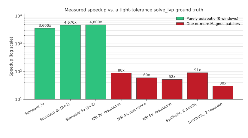
Measured speedup versus a tight-tolerance solve_ivp ground truth across the validation grid (log scale), plotting exactly the numbers in the table above – both come from VALIDATION_GRID in docs/make_figures.py, so they cannot drift apart. Purely adiabatic cases (green) are fastest, since no exact patch is ever computed; cases needing one or more Magnus patches (red) are still 30-90x faster than direct integration, dominated by the (still cheap, since the window is narrow) patch computation and the self-certification refinement loop.

Speedups for the patched cases are smaller than the purely adiabatic ones for a simple reason: a patch means solve_ivp itself is being compared against on a shorter, more tractable sub-problem (the same reason the purely-adiabatic 2ν case reaches the largest speedup of all – it is also the case where solve_ivp is slowest, since nothing shortens its own work). What stays constant across every case is the two things that matter: exact unitarity, at every accuracy setting, and agreement with direct integration well within the package’s standard \(10^{-3}\) target tolerance.

Limitations and scope

• The hybrid strategy requires a genuinely smooth Hamiltonian: the finite-difference Hellmann-Feynman diagnostics assume \(dH/dl\) is well-defined everywhere on the trajectory. A piecewise profile with genuine discontinuities (the Earth’s PREM layers) is out of scope for now; requesting t_slab_edges or density-discontinuity breakpoints disables the hybrid dispatch and falls back to the general method, unconditionally.

• The strategy is fundamentally adaptive (self-certifying): it does not apply when no target tolerance is requested at all (rtol and atol both None), since there is no hybrid analogue of “run once with a fixed slab count.”

magnus.oscprob.osc_prob_sun() and magnus.oscprob.osc_prob_earth() (the fully generic entry points, which accept an arbitrary user-supplied H_func without assuming the separable vacuum-plus-matter-potential structure) also accept strategy, via _osc_prob_hybrid_dispatch_generic – nothing about magnus.adiabatic.hybrid_propagator() requires the separable structure the other wrappers build (it operates on any callable H_func(l)), so the same gating logic (smooth profile, requested tolerance) applies here too, evaluated directly on the user’s own Hamiltonian. In practice this means:

• osc_prob_sun engages the hybrid strategy exactly as readily as the standard/NSI/LIV Sun wrappers, since its density profile has no breakpoints.

• osc_prob_earth almost always falls back to the 'magnus' strategies regardless of what is requested, since t_breakpoints (the PREM layer-boundary crossings) is essentially always non-empty for a real Earth-crossing trajectory – this is the correct, principled consequence of the smoothness requirement above, not a special case written in for osc_prob_earth specifically.

See Methodology for the plain Magnus-expansion machinery this strategy sits alongside, and Code Architecture for where magnus.adiabatic fits into the package’s module layout.