Numerical recipes
What Magνs can compute, with the code that computes it.
Each recipe below is a few lines. Where one is short enough to be worth running on the spot, it is executed when this page is built, so the output shown is what the code actually produced rather than what it produced once. The longer form of every recipe is a notebook, linked beside it; both call the same functions, so there is no third version to drift out of step.
If you are looking for which function rather than how to call it, see
Available Oscillation-Probability Functions, which lays out the whole osc_prob_* family by environment
and flavor count.
One probability
The shortest useful thing the library does: an energy, a baseline, and the oscillation parameters it defaults to.
import numpy as np

import magnus.globaldefs as gd
import magnus.oscprob as oscprob

P = oscprob.osc_prob_3nu_vacuum(1.0*gd.UNIT_GEV, 1300.0*gd.UNIT_KM)

print('P_ee   = %.6f' % np.asarray(P)[0][0])
print('P_mue  = %.6f' % np.asarray(P)[1][0])
P_ee   = 0.928948
P_mue  = 0.031266
The return is the probability matrix, indexed P[nu_i][nu_f]: the initial
flavor first. Pass nu_i and nu_f to get a single channel instead of the
matrix. Full walk-through:
notebook 01.
The evolution operator, for observables built from amplitudes
A probability is a modulus squared. When the observable needs the amplitudes themselves – the content of each mass eigenstate in the state that leaves a dense source, and from it the flavor composition at a detector so far away that the phases have averaged – ask any entry point for the evolution operator alongside the probabilities. The refinement ladder then converges the operator itself, phases included.
import magnus.hamiltonians as hams

OSC = gd.load_nufit_params('NuFIT 6.1')
P, U = oscprob.osc_prob_3nu_matter_exp_density(
    1.0*gd.UNIT_GEV, 5000.0*gd.UNIT_KM, 0.0, 10.0, 1000.0*gd.UNIT_KM,
    density_matter_is_in_g_per_cm3=True, return_evolution_operator=True,
    n_slabs=32, **OSC)

# The mixing matrix in vacuum, the medium past the source; then the
# mass-state content of what leaves, and the flavor content far away
R = hams.pmns_mixing_matrix(OSC['s12'], OSC['s23'], OSC['s13'], OSC['dCP'])
content = abs(R.conj().T @ U)**2
P_far = abs(R)**2 @ content

print('at the edge of the source, P_ee = %.4f' % np.asarray(P)[0][0])
print('far away, phases averaged, P_ee = %.4f' % P_far[0, 0])
at the edge of the source, P_ee = 0.7824
far away, phases averaged, P_ee = 0.4933
P is what the same call returns without the keyword; U is complex and
unitary, indexed U[final, initial], so abs(U)**2.T is P. See
Available Oscillation-Probability Functions for what the keyword does to the engine dispatch and the two
combinations it refuses.
A scan, without a loop
Pass arrays and the whole scan is one call. This is the single most useful thing to know about using Magνs well: the engines batch over the energy axis, and for a position-dependent Hamiltonian the matter profile is then built once for the whole scan rather than once per point.
energies = np.logspace(-1.0, 1.5, 500)*gd.UNIT_GEV
baselines = np.full(500, 1300.0*gd.UNIT_KM)

P = np.asarray(oscprob.osc_prob_3nu_vacuum(energies, baselines))

print('shape returned:', P.shape)
print('P_mue at the first three energies:', np.round(P[:3, 1, 0], 6))
shape returned: (500, 3, 3)
P_mue at the first three energies: [0.339675 0.449521 0.509371]
A batched call returns (n_points, d, d), with the point index first, so
P[:, 1, 0] is \(P_{\mu e}\) along the scan.
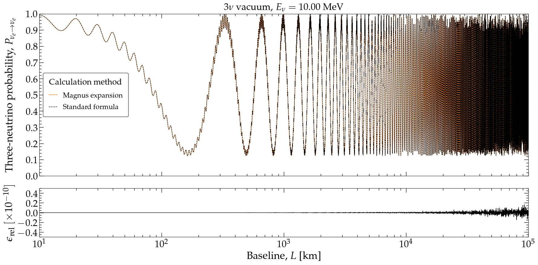
Three-flavor vacuum oscillations.
Writing your own H_func so that it accepts an array of positions is the
other half of this, and is worth a factor of several: see
Writing an H_func that does not cost you a factor of five below.
Through the Earth
Give a zenith angle and the chord, its PREM density profile, and the slab edges aligned with the layer boundaries all follow.
import magnus.earth as earth

costhz = -0.5
L = earth.distance_traveled_inside_earth(costhz)*gd.UNIT_KM

P = np.asarray(oscprob.osc_prob_3nu_earth(10.0*gd.UNIT_GEV, costhz=costhz, L=L))

print('chord   = %.0f km' % (L/gd.UNIT_KM))
print('P_mue   = %.6f' % P[1][0])
chord   = 6371 km
P_mue   = 0.133678
A detector underground is the same call with its depth named. The zenith angle is measured at the detector, so the baseline follows from the geometry and is computed rather than given. A buried detector also sees downward-going neutrinos through its overburden, which a detector on the surface has no path for at all.
depth = 2.0*gd.UNIT_KM

for costhz_det in (-0.5, 1.0):
    L_km = earth.distance_traveled_inside_earth(
        costhz_det, detector_depth=depth/gd.UNIT_KM)
    P_buried = np.asarray(oscprob.osc_prob_3nu_earth(
        10.0*gd.UNIT_GEV, costhz=costhz_det, detector_depth=depth))
    print('costhz = %5.2f: %10.3f km, P_mumu = %.6f'
          % (costhz_det, L_km, P_buried[1][1]))
costhz = -0.50:   6372.998 km, P_mumu = 0.102404
costhz =  1.00:      2.000 km, P_mumu = 1.000000
PREM’s outermost shell is 3 km of global-average ocean, which a detector under
rock or ice is not sitting under. Replace its density with
density_matter_ocean, and its composition with electron_fraction_ocean.
Both matter for a trajectory close to horizontal, which can spend its whole
length inside that shell.
The PREM layer boundaries are inserted as mandatory slab edges automatically, so the quadrature never integrates across a density discontinuity. Notebooks 02 and 03 cover the Earth alongside the other profiles; 06 turns it into an oscillogram.
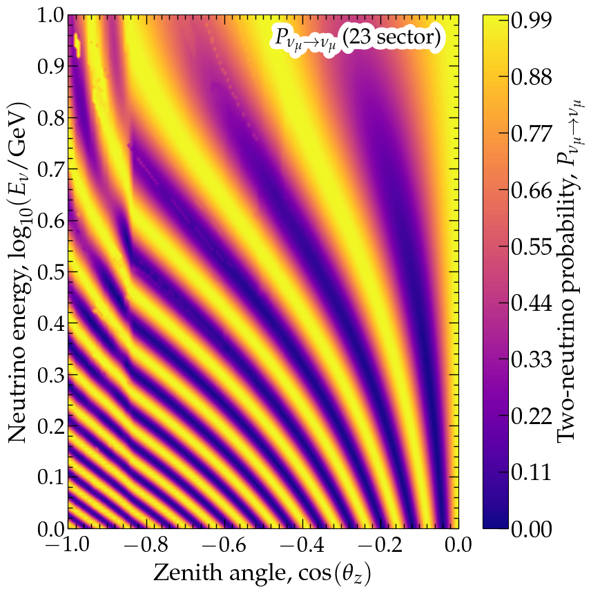
Probability across zenith angle and energy in one call.
A profile of your own
Any callable returning a density as a function of position works. The Sun’s exponential profile ships as a helper, and carries a tag that lets the interaction-picture fast path recognize it. For the Sun itself, twelve published standard solar models ship as well, and the Sun wrappers take them by name (see Standard solar models).
import magnus.matter as matter

profile = matter.exp_density_profile(gd.NUM_DENSITY_E_SUN_CENTRAL,
                                     gd.L_SCALE_SUN)
osc = gd.OSC_PARAMS_PREDEFINED['OSC_PARAMS_DEFAULT']

P = np.asarray(oscprob.osc_prob_matter_std_potential(
    2, profile, 10.0e6, 0.3*gd.SUN_RADIUS*gd.UNIT_KM,
    {'sth': osc['s12'], 'Dm2': osc['D21']},
    L0=0.0, density_is_of_number_of_electrons=True))

print('P_ee = %.6f' % P[0][0])
P_ee = 0.483533
Notebooks 13 and 14 do this with a real tabulated solar model and with a supernova shock front, and are the two places the package’s limits are shown rather than asserted.
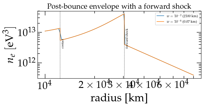
A sharp shock front, where the error is an envelope rather than a phase and averaging does not rescue it.
Phase-averaged probabilities
When the oscillation phase is unresolvable — a source far enough away, or an energy resolution wide enough — the observable is the average, not the instantaneous value. Ask for it directly rather than averaging a scan by hand.
kw = dict(L0=0.0, density_is_of_number_of_electrons=True)
params = {'sth': osc['s12'], 'Dm2': osc['D21']}
L_sun = 0.3*gd.SUN_RADIUS*gd.UNIT_KM

inst = np.asarray(oscprob.osc_prob_matter_std_potential(
    2, profile, 10.0e6, L_sun, params, **kw))
avg = np.asarray(oscprob.osc_prob_matter_std_potential(
    2, profile, 10.0e6, L_sun, params, average=True, **kw))

print('instantaneous P_ee = %.6f' % inst[0][0])
print('phase-averaged     = %.6f' % avg[0][0])
instantaneous P_ee = 0.483533
phase-averaged     = 0.410154
This matters for accuracy as well as for physics: an error that is a phase disappears under averaging, and one that is an envelope does not. See Phase-Averaged Probabilities, and notebook 10.
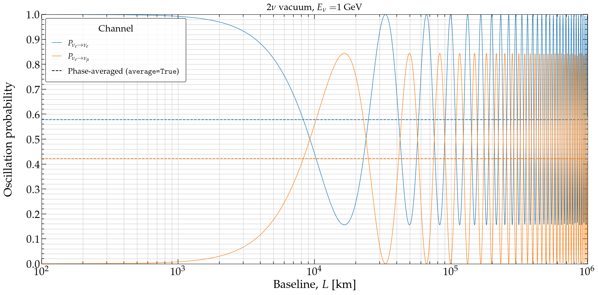
What survives when the phase is unresolvable.
Asking for an accuracy instead of a slab count
n_slabs fixes the discretization, not the error. Pass rtol/atol
instead — they are on by default at 1e-3 — and the slab grid is refined until
two successive levels agree.
info = {}
oscprob.osc_prob_3nu_earth(10.0*gd.UNIT_GEV, costhz=costhz, L=L,
                           rtol=1e-6, atol=1e-6, convergence_info=info)

print('slabs used      : %d' % info['n_slabs'])
print('slab edges used : %d   (PREM boundaries included)' % info['n_slab_edges'])
print('tolerance met   : %s' % info['tolerance_achieved'])
slabs used      : 21
slab edges used : 35   (PREM boundaries included)
tolerance met   : True
Read the tolerance for what it is. It is a stopping criterion, not a
guarantee: the ladder halts when two levels agree, and never estimates the error
of the answer it returns. Usually that is conservative; it is not always. The
rtol entry of magnus.oscprob.osc_prob() says what it does and does not
promise, and What rtol and atol actually control gives the measured detail.
convergence_info reports what the ladder did — including
tolerance_achieved, which is the programmatic form of
ToleranceNotAchievedWarning. There is deliberately no
error estimate in it; the same section explains why.
Choosing a strategy, and seeing which engine answered
strategy='auto' (the default) tries an adiabatic-transport-plus-Magnus-patch
propagator first and falls back silently. 'magnus' reproduces the behavior
of releases before that propagator existed. The difference is not only speed: on
the NSI configurations notebook 12 measures, the fallback is the faster route
and the less accurate one, raising ToleranceNotAchievedWarning rather than
answering quietly.
report = {}
oscprob.osc_prob_matter_std_potential(
    2, profile, 10.0e6, L_sun, params, strategy_info=report, **kw)

print('engine that answered:', report['engine'])
engine that answered: hybrid
Pass strategy_info whenever you want to know which of the engines produced a
number. See Adiabatic + Magnus Hybrid Strategy, and
notebook 12,
which times all three against solve_ivp.
Telling it where the profile is not smooth
High-order quadrature converges at its nominal order only inside a smooth slab. If your profile has a jump or a kink, pass its position as a mandatory slab edge; no number of slabs fixes one that straddles it.
breakpoints = earth.prem_layer_edges_along_chord(costhz)*gd.UNIT_KM

P = oscprob.osc_prob_matter_std_potential(
    3, rho_func, energy, L, osc_params, L0=0.0,
    t_breakpoints=breakpoints)
The Earth entry points do this for you. It is worth doing by hand for a shock front, a castle-wall profile, or a tabulated model with a discontinuous derivative — and on a scan it is an established cure, while on a single point it is not: measured across 18 shock configurations it improved 7 and worsened 11. Notebook 14 is that measurement.
New physics
Non-standard interactions, Lorentz-invariance violation and sterile states are each a different Hermitian matrix in the same slot, so they are the same calculation with a different Hamiltonian.
# NSI: an extra matter potential with off-diagonal couplings
P = oscprob.osc_prob_3nu_earth_nsi(energy, costhz=costhz, L=L,
                                   eps_ee=0.1, eps_em=0.05, eps_et=0.0,
                                   eps_mm=0.0, eps_mt=0.0, eps_tt=0.0)

# LIV: an energy dependence the vacuum term does not have
P = oscprob.osc_prob_3nu_earth_liv(energy, costhz=costhz, L=L,
                                   b1=1.0e-23, b2=0.0, b3=0.0)

# 3+1 sterile: the same machinery at one dimension higher
P = oscprob.osc_prob_4nu_earth(energy, costhz=costhz, L=L,
                               s12=s12, s23=s23, s13=s13, d13=d13,
                               s14=0.1, s24=0.1, s34=0.0,
                               D21=D21, D31=D31, D41=1.0)
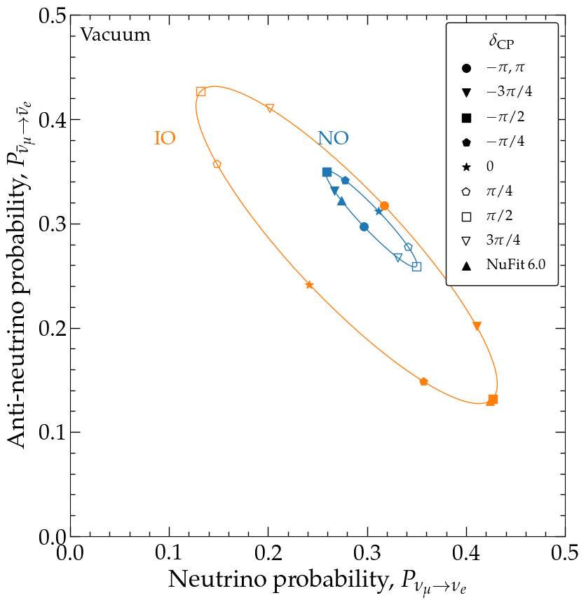
Neutrino against antineutrino as the CP phase runs, for both mass orderings.
Writing an H_func that does not cost you a factor of five
If you supply your own Hamiltonian, the single largest factor under your control is whether it can be evaluated for many positions at once. The engine samples it at every quadrature node of every slab — often a few hundred positions for one probability, repeated at each refinement level.
# Slow: one position at a time
def H_func(l):
    VCC = matter.VCC_func(l, num_density_e_func)
    return (1.0/energy)*h_vac + hamiltonians.hamiltonian_3nu_matter(VCC)

# Fast: the same physics, all positions at once
e00 = np.diag([1.0, 0.0, 0.0])
def H_func(l):
    l = np.asarray(l, dtype=float)
    VCC = vcc_of(l)                       # returns an array
    return (1.0/energy)*h_vac + VCC[..., None, None]*e00
The trailing [..., None, None] is the whole trick: it turns one potential per
position into a stack of matrices, so NumPy broadcasts instead of Python looping.
Measured at 4.6x on a 3ν exponential-density profile, with bit-identical
output. A scalar-only H_func raises
ScalarHamiltonianWarning once per session, naming the fix.
Where to go next
Tutorial notebooks — the same calculations with the reasoning around them.
Available Oscillation-Probability Functions — every
osc_prob_*function, by environment and flavor.Methodology — what the Magnus expansion is and why it is unitary at any order.
Engines and dispatch — which engine answers a call, and how the choice is made.
Performance — the constants and the populations they were measured on.
Accuracy and diagnostics — what each safeguard cannot do, and what every warning means.
Command-Line Calculator — the same calculations from a shell.