Against other codes

Magνs is not the fastest way to compute every oscillation probability, and this page says where it is not. Everything below is measured in notebook 25, with every code timed in one process on one machine and refereed by a method that is neither code’s. The frozen datasets it draws on live in notebooks/external_*.json.

Two codes are compared throughout: NuOscProbExact [Bus19], which solves each slab of constant density in closed form, and nuSQuIDS [ArguellesSW22, DSW15], which integrates the density-matrix evolution.

Warning

Absolute timings are a property of the machine and are worth little on their own. Read the ratios within a row, and read a tolerance sweep only within one code’s own curve. “Code A is faster than code B” does not survive a change of hardware; “tightening this dial costs 20% and buys four orders of magnitude” does.

The boundary, stated once 

Where a closed form exists and the accumulated phase is large, use the closed form. An exact algebraic solution beats a truncated series; that is arithmetic, not a defect in either code. Constant density, piecewise-constant PREM and standard three-flavor propagation are precisely what closed forms are built for, and on those Magνs does not win on cost.

What Magνs buys is everything that is not that: accuracy past the point where a piecewise-constant discretization stalls, an arbitrary varying profile, a Hamiltonian nobody has diagonalized, five flavors, and observables that are returned rather than reconstructed.

Which one should I use?

Magνs integrates a Hamiltonian across each slab, which is what lets it follow a density that changes as the neutrino moves. That machinery is wasted — and slower than the alternative — when the Hamiltonian does not change at all.

Reach for NuOscProbExact when the Hamiltonian is constant, or piecewise constant. It expands the Hamiltonian and the evolution operator in the SU(2), SU(3) and SU(4) bases, which gives a closed form rather than a numerical integration: exact up to floating-point round-off, and with no slab count to choose.

Situation	Use this	Because
Constant density	NuOscProbExact	One closed form, no integration
Piecewise constant, tens of layers — the Earth through PREM	NuOscProbExact	Each layer solved exactly, operators multiplied
Smoothly varying, slow against the oscillation	Either	Slabbing converges quickly
Smoothly varying, fast against the oscillation — the Sun, adiabatic MSW	Magνs	Slabbing needs \(\sim 10^4\) steps per resonance crossing
A front resolved across many slabs — a shock from a simulation snapshot	Magνs	Smooth on the slab scale, so fourth order beats second
A front thin against the oscillation length — a real hydrodynamic shock	NuOscProbExact	To any sampling method that is a jump, which is a closed form’s home ground
A kink, a tabulated profile	Magνs	`t_breakpoints` puts a slab edge on the discontinuity
More than four flavors	Magνs	The SU(N) expansions stop at SU(4); Magνs has no ceiling
Genuinely open systems: decay, decoherence	Neither	Needs a Lindblad solver, not a unitary one

The two packages share conventions, units and parameter defaults deliberately, so a calculation can be moved between them as a cross-check. That is worth doing: agreement between two methods with different failure modes is stronger evidence than either one’s internal convergence check.

Constant density 

Both codes are exact here, to round-off:

Route	Total [s]	µs/point	max \|P − exact\|
Magνs, batched wrapper	0.0006	9.72	9.0e-17
Magνs, one call per energy	0.0057	95.06	9.0e-17
NuOscProbExact, looped	0.0009	14.32	4.9e-16
NuOscProbExact, batched	0.0001	1.34	4.9e-16

1300 km at 2.848 g/cm³, 60 energies from 0.6 to 20 GeV. The lesson here is about batching, not about codes: either code called one energy at a time costs about an order of magnitude more than the same physics asked for in one call.

PREM, three flavors 

An Earth chord at \(\cos\theta_z = -0.85\) (10 831 km), refereed by a Richardson-extrapolated slab product whose own residual discretization error is 4.3e-07 — nothing below that line is resolvable by this comparison.

Refined against itself, each code reaches:

	Magνs	NuOscProbExact
Best accuracy reached	3.3e-10	5.6e-05
Cost per call	~20× more	~20× less

The residual between the two codes is 4.1e-04, which is the same order as the looser of the two curves — so most of it is NuOscProbExact’s discretization rather than a disagreement about physics. A residual far above both curves would have meant a convention mismatch instead, and that is the check worth making before concluding anything from a cross-code difference.

PREM, 3+1 

The most expensive case for Magνs in the whole comparison, and — once the referee was corrected — not the least accurate one. The two axes point in opposite directions, so they are worth separating.

Cost: NuOscProbExact, by about 400×. 56 000 µs per probability against 127. The cost does not fall when the tolerance is loosened, and that flatness is the diagnosis: the refinement ladder is not converging and stopping, it is running to its slab ceiling. An eV-scale \(\Delta m^2_{41}\) over an 11 000 km chord accumulates a phase whose required slab width is below what the ladder will reach, which is why a MagnusConvergenceWarning appears on every row.

Accuracy: Magνs, and it reaches the floor of the measurement. Its residual against the referee is 4.5e-08, below the referee’s own discretization error of 4.1e-07 — so the honest statement is that Magνs agrees with the referee to within the referee’s uncertainty, and this comparison cannot resolve it further. NuOscProbExact sits at 2.6e-04, some six hundred times above that floor, and its convergence is not monotonic: 32 slabs per segment is worse than 8. Non-monotonic convergence is the signature of a discretization whose edges straddle structure they do not resolve, and it means there is no setting of that dial to read off as “converged”.

Note

A convergence warning is a statement about evidence, not about error. Magνs warns on every row here and is right to — the answer is not backed by a convergence argument. It is also the most accurate answer on the plot. The two come apart exactly here.

A smooth profile: where each method runs out 

On a smooth exponential profile the comparison is no longer about cost but about reach. Composing slabs is second order in the slab width, so halving it buys a factor of four; the Gauss–Legendre Magnus expansion is fourth order and buys sixteen. More importantly the slab product has a floor:

Exponential profile, 3ν	Best error	At
NuOscProbExact	2.5e-11, then rises	16 384 slabs; 32 768 is worse
Magνs	2.9e-13	tightest tolerance

Past about 16 000 slabs the round-off of composing that many matrix products costs more than another halving of the width buys. No setting reaches below that floor. At five flavors there is no comparison to draw at all — NuOscProbExact has no five-flavor route — which is the other half of the same point.

The Sun: an observable the others do not offer 

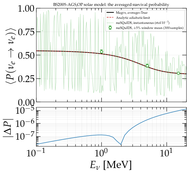
The averaged solar survival probability against the instantaneous one — The averaged solar survival probability, returned directly. The instantaneous probability another code returns is the trace thrashing between 0.15 and 0.9 — it is not the observable.

The model is the tabulated BS2005-AGS,OP solar profile [BSB05]. A neutrino leaving the Sun accumulates some 13 000 radians of phase at 5 MeV, so the instantaneous survival probability at the surface is neither measurable nor stable: neighboring energies land anywhere between 0.15 and 0.9. What a solar experiment measures is the phase-averaged probability, and average=True returns it directly — 40 averaged energies in about 0.7 s, matching the analytic adiabatic limit to 1.3e-05.

nuSQuIDS needs about ten minutes merely to reach the solver tolerance at which its output is a probability at all, and then a further factor of N to average the phase away:

`rel_error`	Seconds	P over all flavors	A probability?
1e-04	160.8	−1.19 … 3.09	no
1e-05	251.3	−0.011 … 1.007	no
1e-06	568.1	0.0002 … 0.979	yes
1e-07	1078.2	0.0001 … 0.979	yes

Warning

The obvious guard passes on every one of those rows. Summing the flavor probabilities and checking they come to one holds to 1e-16 even where the survival probability reaches 2.83. That is not a bug in the guard: nuSQuIDS evolves the density matrix in an SU(3) basis whose identity component is the trace, so the flavor sum is conserved by construction however badly the traceless components are integrated. A structural invariant cannot test the thing it is built into. The check that does bite is each probability lying in \([0, 1]\).

Neither of the other codes offers an averaging flag. This is a different algorithm for the question a solar experiment actually asks, not the same algorithm run faster.

A supernova shock: the width of the front decides 

The same physics, the same codes, and the winner changes with one parameter — how sharp the front is:

Front width	Magνs	NuOscProbExact
0.07 km (sharp)	2.4e-09	1.4e-09
70 km (smooth)	9.6e-10	5.6e-06

On a sharp front the profile is piecewise constant, which is the closed form’s home ground and it matches Magνs there at a fraction of the cost. Widen the front and the same closed form stalls four orders of magnitude higher, because it is now approximating a smooth function with steps. Neither result is about implementation quality; both are about which method the problem belongs to.

Summary 

Case	Outcome
Constant density, exactness	Both ~1e-16
Constant density, speed	Comparable batched; both ~10× slower called one energy at a time
PREM 3ν, cost	NuOscProbExact by ~20×
PREM 3ν, accuracy reachable	Magνs to 3e-10; the closed form stalls near 6e-05
PREM 3+1, cost	NuOscProbExact by ~400×, and Magνs warns
PREM 3+1, accuracy reachable	Magνs, to the referee’s own floor (4e-07); the closed form stalls near 3e-04, non-monotonically
Smooth profile, reach	Slab product floors at 2.5e-11 and then rises; Magνs continues to 2.9e-13
Five flavors	Magνs only — NuOscProbExact has no route
Solar averaged observable	Magνs returns it directly; nothing else here offers it
Supernova shock	The width of the front decides, not the flavor content

The table has no winner in it. It has a boundary.

Before comparing any two codes’ numbers 

Check that they agree in vacuum first. If they do not, the disagreement is in the solvers. If they agree in vacuum and disagree in matter, it is in the conventions — a matter-potential factor, an electron fraction, a channel index — and no amount of tolerance will close it. Notebook 25 spends a whole section on a conventions trap for this reason: a 1% difference in \(V_{\rm CC}\) reads exactly like an accuracy difference until you look.