Phase-Averaged (Decohered) Probabilities

This page documents the average keyword accepted by magnus.oscprob.osc_prob_vacuum(), magnus.oscprob.osc_prob_matter_std_potential(), magnus.oscprob.osc_prob_matter_nsi() and magnus.oscprob.osc_prob_liv() – and therefore, through the shared **kwargs chain, by every osc_prob_{2,3,4,5}nu_* wrapper built on them – together with the module that implements it, magnus.avgprob. See Adiabatic + Magnus Hybrid Strategy for the position-dependent machinery this reuses, and Methodology for the plain Magnus engine both sit alongside.

The problem: a phase nobody can resolve

A neutrino from an astrophysical source arrives with an oscillation phase

\[\Delta \phi = \frac{\Delta m^2 L}{2E} \simeq 1.27 \times \frac{\Delta m^2/\text{eV}^2 \times L/\text{km}} {E/\text{GeV}}\]

of order \(10^{15}\) for a TeV neutrino from 100 Mpc away. No ingredient of that number is known to anything close to the precision the phase would demand: not the source distance, not the size of the production region, and not the detector’s energy resolution. Whatever the true phase is, the measurement integrates over many complete cycles of it.

Computing such a probability by propagation is therefore doubly unattractive. It is expensive – resolving \(10^{15}\) radians is exactly the regime that defeats slab refinement – and it is pointless, because every oscillatory term is about to be averaged away by the integration the measurement performs anyway.

The averaged limit

Write the amplitude in the basis that diagonalizes the Hamiltonian, \(H = V \,\mathrm{diag}(\lambda_i)\, V^\dagger\):

\[A(\nu_\alpha \to \nu_\beta) = \sum_i V^*_{\alpha i} V_{\beta i}\, e^{-i \lambda_i L} .\]

The probability \(|A|^2\) contains a diagonal part and interference terms carrying \(e^{-i(\lambda_i - \lambda_j)L}\). Averaging over the phase leaves only the terms whose phase does not vary:

\[\boxed{\;P(\nu_\alpha \to \nu_\beta) = \sum_i |V_{\alpha i}|^2\, |V_{\beta i}|^2\;}\]

This is not an approximation to be refined: it is the exact \(L/E \to \infty\) limit, and it costs one matrix product rather than an integration. Three properties follow immediately and are worth stating, because each surprises someone eventually:

The result is symmetric in \(\alpha \leftrightarrow \beta\), so the averaged probability is the same in both directions.
It is identical for neutrinos and antineutrinos, since \(|V^*|^2 = |V|^2\). CP violation does not survive the average, even though \(\delta_{\rm CP}\) still enters through the magnitudes \(|V_{\alpha i}|\).
For vacuum oscillations it does not depend on energy or baseline at all: scaling \(H\) by \(1/E\) leaves its eigenvectors untouched, so a single matrix serves an entire flux calculation.

Coherence is a physical question, not a numerical one

The boxed expression assumes every relative phase has averaged away. That is a statement about pairs of eigenvalues, not about the spectrum as a whole: the pair \((i,j)\) decoheres only once \((\lambda_i - \lambda_j)L\) has swept through many cycles. Two eigenvalues close enough to keep their relative phase fixed stay coherent, and their cross term survives.

magnus.avgprob therefore groups the spectrum into blocks of mutually coherent eigenvalues and sums coherently inside each block,

\[P(\nu_\alpha \to \nu_\beta) = \sum_{b} \Big| \sum_{i \in b} V^*_{\alpha i} V_{\beta i} \Big|^2 ,\]

which reduces to the boxed expression when every block is a singleton. The distinction is not academic. A sterile state with a small \(\Delta m^2_{41}\), or any exactly degenerate spectrum, makes the naive sum quietly wrong: with all eigenvalues equal the correct answer is the identity – nothing oscillates at all – while the naive sum returns a spurious mixture.

The same per-pair phase decides whether an averaged expression applies at all. A pair is in one of three regimes:

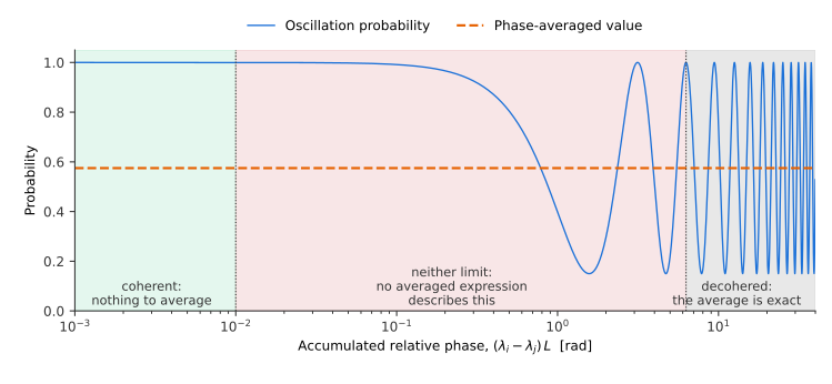
The coherent, intermediate and decohered regimes of a pair of eigenvalues

far below magnus.avgprob.COHERENCE_PHASE_THRESHOLD, the relative phase has barely advanced: the pair is coherent and there is nothing to average;
far above magnus.avgprob.DECOHERENCE_PHASE_THRESHOLD, the cross term has averaged away and the boxed expression is exact;
in between, neither statement holds, and no averaged expression describes the result. The honest quantity there is the oscillation probability itself.

magnus.avgprob.coherence_report() names the pairs in that middle band, and the callers in magnus.oscprob raise magnus.oscprob.PhaseAveragingWarning rather than return a number the physics does not support. Asking for an averaged probability at a 1000 km beamline does exactly this: the solar pair has accumulated about 0.2 radians there, and the averaged expression disagrees with the true probability by tenths.

Position-dependent Hamiltonians

When the Hamiltonian varies along the trajectory there is no single eigenbasis to decohere in. A neutrino produced at \(l_0\) decoheres in the eigenbasis there, is carried along the levels of the instantaneous Hamiltonian, and is detected in the eigenbasis at \(l_1\):

\[P(\nu_\alpha \to \nu_\beta) = \sum_{ij} |V_{\alpha i}(l_0)|^2 \, P^{\rm cross}_{ij} \, |V_{\beta j}(l_1)|^2 ,\]

the standard MSW-plus-decoherence result, generalized here to any number of levels and any number of crossings. \(P^{\rm cross}\) is the probability of ending on level \(j\) having started on level \(i\). Adiabatic evolution keeps a neutrino on its level, so \(P^{\rm cross}\) is the identity wherever the adiabatic approximation holds, and departs from it only across a non-adiabatic window.

Those windows are located with the Hellmann-Feynman diagnostic of magnus.adiabatic (see Adiabatic + Magnus Hybrid Strategy), and the transfer across each one is computed with that module’s own convergence-checked Magnus patch – not with a Landau-Zener formula. The result is an exact treatment of the crossing rather than an asymptotic approximation to it. As a check, the computed hop probability reproduces the analytic Landau-Zener value \(\exp(-2\pi\epsilon^2/|d\Delta/dl|)\) to a few parts in a thousand for a linear crossing, with nothing in the implementation assuming that formula:

Coupling \(\epsilon\)	Computed hop probability	Landau-Zener	Difference
\(10^{-4}\)	0.9382	0.9391	0.1%
\(3\times10^{-4}\)	0.5665	0.5680	0.3%

Two conditions have to hold for the expression above to mean anything, and magnus.avgprob.averaged_probabilities_adiabatic() checks both rather than assuming them. The levels must have decohered from each other by the time of detection; and if there is more than one crossing, they must also have decohered between crossings, since otherwise composing the crossings as probabilities – rather than as amplitudes – discards interference that is still present. Both are returned in the report, naming the stretch and the pair at issue.

When there is no closed form

A profile with discontinuities – the PREM layer boundaries an Earth-crossing trajectory steps through – has no instantaneous eigenbasis to decohere in, so neither construction above applies. There, average=True propagates the probability for real across an energy window and averages over it (magnus.avgprob.averaged_probabilities_numerically()).

This returns a different quantity from the other two paths. They return the exact \(L/E \to \infty\) limit, which needs no window; this returns the average over one particular window, and the answer depends on its width. The default width, magnus.avgprob.AVG_DEFAULT_ENERGY_SPREAD, is 10% – the order of a real detector’s energy resolution – and every use of it raises magnus.oscprob.PhaseAveragingWarning naming the width, the number of samples, and the standard error of the resulting mean, so the figure is never silently dependent on a constant the caller did not choose. Callers with a known resolution should pass their own.

Cost

Case	Method	Exact?	Cost
Vacuum, constant density (and their NSI/LIV variants)	Closed form	Yes	~20 \(\mu\)s
Exponential density, Sun (and their NSI/LIV variants)	Adiabatic + crossing matrix	Yes, in that limit	~0.07 s
Earth (PREM)	Sampled over an energy window	No – window-dependent	~0.1 s

For comparison, obtaining the same vacuum number by averaging the engine numerically over 2001 energies takes about 0.25 s and is an approximation, against 20 \(\mu\)s for an exact answer.

Usage

import numpy as np

import magnus.oscprob as oscprob
import magnus.globaldefs as gd

# load_nufit_params returns just the six mixing parameters; the
# OSC_PARAMS_PREDEFINED entries also carry 'name'/'description' strings,
# which the propagation machinery would reject.
osc = gd.load_nufit_params('NuFIT 6.1')

P = oscprob.osc_prob_3nu_vacuum(1.0*gd.UNIT_TEV, 1.0e8*gd.UNIT_KM,
                                average=True, **osc)
np.round(np.asarray(P), 4)

array([[0.5481, 0.2155, 0.2364],
       [0.2155, 0.4071, 0.3774],
       [0.2364, 0.3774, 0.3862]])

The most quoted consequence of averaged astrophysical oscillations follows in one line: a source producing the pion-decay composition \((1:2:0)\) delivers something close to equipartition at Earth.

at_source = np.array([1.0, 2.0, 0.0])/3.0
at_earth = at_source @ np.asarray(P)
np.round(at_earth*3.0, 3)

array([0.979, 1.03 , 0.991])

Am I computing the wrong thing? `strategy_info['sampling']`

The hardest part of this page in practice is not the mathematics – it is noticing that it applies to you. A scan of instantaneous probabilities over a long trajectory returns perfectly correct numbers, and they can still be the wrong quantity, because the observable is an average over a phase nobody resolves.

Every osc_prob_* entry point that accepts strategy_info now reports how coarsely the request samples the oscillation it is computing:

info = {}
P = magnus.oscprob.osc_prob_3nu_sun(energy, L, info_kwargs..., strategy_info=info)
info['sampling']
# {'oscillation_length': 2.53e+10,   'cycles_over_trajectory': 1.32e+04,
#  'spacing': 3.82e+13,              'cycles_per_step': 1.51e+03,
#  'nyquist_points': 26446,          'aliased': True}

cycles_per_step is the number to read. Above about 0.5 the scan takes less than two samples per oscillation, so the returned array cannot represent the oscillation and must not be plotted or interpolated as a curve – the individual values are right, the curve through them is an artefact. nyquist_points says how many baselines would be needed to sample it properly.

Those numbers are usually stark. Measured over the physically-motivated profile families in docs/dev/adversarial_batteries/:

trajectory	oscillations across it	baselines for Nyquist
Earth chord	~430	861
Solar, one scale height	~2200	4 390
Supernova ray	~37 000	73 392

This is reported and never warned about, deliberately. The Nyquist criterion is objectively correct and would fire on 44 of 45 realistic scan sizes – a warning firing on 98 % of calls is noise however right each firing is, and it would teach users to silence a category that also carries genuine discontinuity warnings. The measurement behind that decision is adversarial_batteries/alias_fp.py.

The report costs eigenvalues at eight points along the trajectory, so it is computed only when ``strategy_info`` is supplied: callers who do not ask pay nothing, and callers who do pay 5.5 % of the cheapest scan measured and under 0.1 % of a substantial one.

When aliased is True, the question worth asking is whether you wanted the average all along. If you did, average=True or magnus.avgprob gives it exactly, in one matrix product rather than an integration. magnus.avgprob.coherence_report() will say whether the averaged expression is valid for your spectrum and baseline, or whether some pair sits in the middle regime where neither limit holds.

How much does the phase actually matter?

It depends on the profile, and the difference is measurable rather than a matter of taste. Averaging an instantaneous scan over six oscillation lengths and comparing against a solve_ivp reference (adversarial_batteries/avg_check.py and avg_check2.py):

configuration	instantaneous	averaged	reduction
Solar model, d = 2, 5 MeV	1.380e-03	2.603e-05	53x
Supernova turbulence, 45 MeV	1.701e-03	1.565e-04	23x
Supernova shock, 70 km front	1.095e-03	9.773e-04	2x
Supernova shock, 0.07 km front	2.033e-01	2.135e-01	3x

The reduction factor separates two physically different things with no overlap. Errors that shrink by more than twentyfold are phase: a smooth or oscillatory profile perturbs when the oscillation is, and no observable sees that. Errors that barely move are envelope: a shock front changes the adiabaticity of the level crossing, so it moves the conversion probability itself, and averaging cannot remove it. A large instantaneous error on a smooth profile is therefore usually harmless, and a modest one across a sharp front usually is not.

Limitations and scope

The averaged limit is a statement about a measurement that integrates over phase. It is not a model of quantum decoherence: there is no dissipative term here, and no density-matrix evolution. See the “When is Magνs not the right tool?” section of Magνs: Neutrino Oscillations via the Magnus Expansion.
Non-adiabatic crossings are handled, but composing more than one assumes the levels dephase between them. That assumption is checked and reported, not silently made.
The Earth/PREM path is a windowed average rather than a limit, as described above.

See Available Oscillation-Probability Functions and the API reference for the full listing of magnus.avgprob.