Bi-probability plot

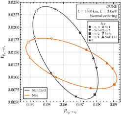
Bi-probability plot at the DUNE baseline. Antineutrino against neutrino appearance probability, as \(\delta_{\rm CP}\) varies, at 2 GeV, over the 1300-km baseline of DUNE, through matter of constant density 3 g cm\(^{-3}\). The two curves are for standard oscillations and for oscillations with non-standard interactions (NSI), with the couplings of Figure New physics along an Earth chord: \(\varepsilon_{ee} = 0.10\), \(\varepsilon_{e\mu} = 0.05\), and \(\varepsilon_{\mu\tau} = 0.03\). Markers show selected values of \(\delta_{\rm CP}\) and the NuFIT 6.1 best fit. Listing Bi-probability curves at the DUNE baseline computes the curves. See notebooks #05 and #28.

Figure Bi-probability plot at the DUNE baseline shows a bi-probability plot  [MN01]: the antineutrino appearance probability against the neutrino one, at one energy and baseline. Each value of \(\delta_{\rm CP}\) gives one point, so taking the phase through its range traces a closed curve. The figure draws two curves, for standard oscillations and for oscillations with non-standard interactions, and they cross at four points. At each crossing, one measurement of the two probabilities fits both cases; e.g., at \(P_{\nu_\mu \to \nu_e} = 0.080\) and \(P_{\bar{\nu}_\mu \to \bar{\nu}_e} = 0.008\), it fits the standard case with \(\delta_{\rm CP} = -0.58\pi\) and the non-standard one with \(\delta_{\rm CP} = -0.31\pi\). A new interaction can then pass for a shift in the phase. Separating the two takes a second measurement, at another energy or baseline.

Listing Bi-probability curves at the DUNE baseline computes the two curves. Both come from the same loop over \(\delta_{\rm CP}\): one calls the standard wrapper, the other the wrapper with non-standard interactions. Any two hypotheses that a measurement might confuse can be compared in the same way, by changing the wrapper or its parameters; notebook #05, e.g., compares the two mass orderings.

Bi-probability curves at the DUNE baseline. The two curves of Figure Bi-probability plot at the DUNE baseline. The function locus takes a wrapper once around \(\delta_{\rm CP}\), computing the neutrino and the antineutrino probability at each of 181 values. The oscillation parameters are the default set, NuFIT 6.1. No tolerance is passed: the Hamiltonian is constant, so the Magnus expansion ends at its first term, and the result is exact. The curves are drawn twice: first with plotting.plot_biprobability, in the preset style of Pre-packaged plotting routines, then with matplotlib directly. See notebooks #05 and #28.

import numpy as np
import matplotlib.pyplot as plt
import magnus.oscprob as oscprob
import magnus.globaldefs as gd
import magnus.plotting as plotting

# DUNE: 2 GeV, 1300 km; a crust-like 3 g/cm^3
E, L, rho = 2.0*gd.UNIT_GEV, 1300.0*gd.UNIT_KM, 3.0
kw = dict(nu_i=gd.NUMU, nu_f=gd.NUE,
          density_matter_is_in_g_per_cm3=True)
eps = dict(eps_ee=0.10, eps_em=0.05, eps_mt=0.03)
std = oscprob.osc_prob_3nu_matter_constant_density
nsi = oscprob.osc_prob_3nu_matter_nsi_constant_density

def locus(wrapper, **couplings):
    """(P_mu e, P_mubar ebar) once around delta_CP."""
    out = []
    for dcp in np.linspace(-np.pi, np.pi, 181):
        P = [wrapper(E, L, rho, nubar=nubar, dCP=dcp,
                     **couplings, **kw)
             for nubar in (False, True)]
        out.append(P)
    return np.array(out)

P_std = locus(std)
P_nsi = locus(nsi, **eps)

# With the shipped plotter
fig, ax = plotting.plot_biprobability(
    [P_std[:, 0], P_nsi[:, 0]],
    [P_std[:, 1], P_nsi[:, 1]],
    labels=['Standard', 'NSI'])

# With matplotlib directly
fig, ax = plt.subplots()
for P, label in ((P_std, 'Standard'), (P_nsi, 'NSI')):
    ax.plot(P[:, 0], P[:, 1], label=label)
ax.set_xlabel(r'$P_{\nu_\mu \to \nu_e}$')
ax.set_ylabel(r'$P_{\bar\nu_\mu \to \bar\nu_e}$')
ax.legend()