Assorted long examples
A cavity in the Earth’s crust
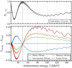
A cavity in the Earth’s crust. Effect of a cavity in the Earth’s crust on the \(\bar{\nu}_e\) survival probability over a baseline of \(1\,500\) km, computed with Magνs, after Ref. [ArguellesBG15]. Top: the crust alone, uniform at 3.3 g cm\(^{-3}\) with \(Y_e = 0.5\). Bottom: the change that four cavities make to it, each centered on the baseline, with the density and width its label gives. The water cavity carries \(Y_e = 0.555\), the other three 0.5. The dashed line marks 49 MeV, where the crust curve peaks. The beam of Ref. [ArguellesBG15] spans 5–150 MeV; below 25 MeV, the oscillation is too rapid to draw. Listing A cavity in the Earth’s crust computes every curve. See notebook #28.
A cavity in the Earth’s crust. A cavity search in the Earth’s crust, after Ref. [ArguellesBG15]: the \(\bar{\nu}_e\) survival probability over \(1\,500\) km of Earth’s crust, with and without a cavity of different density centered on the baseline. A cavity is a density profile with two walls, whose positions are declared as breakpoints so that the refinement ladder runs inside the cavity. See notebook #28.
import numpy as np
import magnus.oscprob as oscprob
import magnus.matter as matter
import magnus.globaldefs as gd

L0 = 1500.0                     # km, source to detector
RHO_CRUST, YE_CRUST = 3.3, 0.5  # Near PREM's crust
E = np.linspace(25.0, 150.0, 2500)*gd.UNIT_MEV
osc = gd.load_nufit_params('NuFIT 6.1')
kw = dict(osc_params=osc, L0=0.0, nu_i=gd.NUE,
          nu_f=gd.NUE, nubar=True, rtol=1.0e-8,
          atol=1.0e-10,
          density_is_of_number_of_electrons=True)

def n_e(rho, ye):
    """Electron density [eV^3] of uniform matter."""
    return matter.num_density_e_func(
        0.0, lambda _: rho, electron_fraction=ye,
        ratio_number_neutrons_to_protons=(1.0-ye)/ye,
        density_matter_is_in_g_per_cm3=True)

NE_CRUST = n_e(RHO_CRUST, YE_CRUST)

def cavity(rho, ye, w):
    """Crust holding a cavity of width w, centered."""
    d = (L0 - w)/2.0
    ne_in = n_e(rho, ye)

    def profile(l):
        x = np.asarray(l, dtype=float)/gd.UNIT_KM
        return NE_CRUST + (ne_in - NE_CRUST) \
            *((x >= d) & (x <= d + w))

    return profile, np.array([d, d + w])*gd.UNIT_KM

# An empty crust needs no profile, only a number
P0 = oscprob.osc_prob_matter_std_potential(
    3, NE_CRUST, E, L0*gd.UNIT_KM, **kw)

# Water, iron, a mineral deposit, a zone of faults:
# (rho, Y_e, w) for each
CASES = [(1.0, 0.555, 250.0), (5.0, 0.5, 250.0),
         (10.0, 0.5, 100.0), (25.0, 0.5, 50.0)]
dP = []
for rho, ye, w in CASES:
    profile, walls = cavity(rho, ye, w)
    # The two walls are density jumps: declare them
    P = oscprob.osc_prob_matter_std_potential(
        3, profile, E, L0*gd.UNIT_KM,
        t_breakpoints=walls, **kw)
    dP.append(P - P0)
A region of anomalous density along the path of a neutrino through an otherwise uniform medium changes the oscillation probability measured at the far end. Using neutrinos to explore the interior of the Earth was proposed decades ago [DRGWC83, ETC86]; oscillations in matter offer one way to do it (see, e.g., Ref. [Win06]). Reference [ArguellesBG15] applied this to a search for cavities in the Earth’s crust. We use Magνs to implement the setup of Ref. [ArguellesBG15]: a low-energy \(\bar{\nu}_e\) beam crossing \(1\,500\) km of crust, with the survival probability measured from 5 to 150 MeV. The example is illustrative; we do not claim that such an experiment is feasible.
Listing A cavity in the Earth’s crust sets this up. The crust is uniform at 3.3 g cm\(^{-3}\) with \(Y_e = 0.5\), a round value close to the 0.4952 of the PREM crust. A cavity is a slab of different density, centered on the baseline. We show four cavities, with the densities and labels of Ref. [ArguellesBG15]: water at 1 g cm\(^{-3}\) with \(Y_e = 0.555\), an iron-banded formation at 5 g cm\(^{-3}\), a mineral deposit at 10 g cm\(^{-3}\), and a zone of seismic faults at 25 g cm\(^{-3}\); the last two are denser than any natural rock, and serve to show how the effect grows with density. Their widths along the path range from 250 to 50 km, the densest being the narrowest. Each wall of a cavity is a density jump, so we pass the positions of both walls to the scenario function via t_breakpoints; this places a slab edge on each wall, so that no slab straddles a jump (Numerical recipes).
Figure A cavity in the Earth’s crust shows the resulting probabilities. Without a cavity, the survival probability peaks at 0.9997 near 49 MeV, where the oscillation driven by \(\Delta m^2_{21}\) completes half a cycle (the peak would reach exactly 1 if \(\theta_{13}\) were zero). A cavity shifts this peak along the energy axis, leaving its shape almost unchanged. A denser cavity adds column density and pushes the peak to higher energy; a lighter one removes column density and pulls it to lower energy. Therefore, just below the peak of the crust curve, a denser cavity lowers the probability, and just above it, raises it; a lighter cavity does the opposite. Every curve of the change crosses zero between the peak of the crust curve and that of the cavity curve, between 48.2 and 49.5 MeV.
Figure A beam swept across a buried body sweeps the beam across a buried body. The source stays fixed and the baseline keeps its length of \(1\,500\) km; only the direction of the beam changes, by an angle \(\alpha\). The body is a sphere of radius 125 km at the density of the mineral deposit, 10 g cm\(^{-3}\), centered 750 km from the source along the baseline at \(\alpha = 0\). (Ref. [ArguellesBG15] uses elliptical cavities, but a sphere makes the same point.) The beam crosses the body only for \(\lvert \alpha \rvert < 9.59^\circ\); the width it crosses is largest, 250 km, at \(\alpha = 0\), and falls to zero at the edges of that band.
The change in probability follows that width: it is largest near \(\alpha = 0\) and fades toward the edges of the band. Outside the band, the beam misses the body, the profile is the uniform crust, and the change is exactly zero. The sweep is what separates a large, light body from a small, dense one. Along a single direction, the probability depends mainly on the excess column density, i.e., the density contrast times the width, so density and width cannot be told apart; the angular width of the band fixes the size of the body independently. Listing A beam swept across a buried body computes the map.
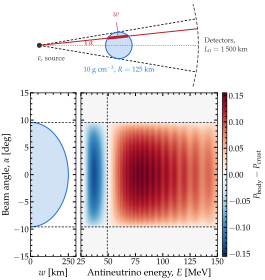
A beam swept across a buried body. Top: the geometry. The beam leaves the source at an angle \(\alpha\) and reaches a detector on the dashed arc, \(1\,500\) km away. The two dashed straight lines are the beams tangent to the body, at \(\alpha = \pm 9.59^\circ\). The beam crosses a width \(w\) of the body. Bottom left: width against angle, i.e., the cavity’s silhouette. Bottom right: change in probability over energy and angle. The dashed vertical line marks the \(49\) MeV of Figure A cavity in the Earth’s crust. Listing A beam swept across a buried body computes the map. See notebook #28.
A beam swept across a buried body. The map of Figure A beam swept across a buried body, which reuses n_e, NE_CRUST, L0, and kw from Listing A cavity in the Earth’s crust. For each beam angle, crossing finds where the chord enters and leaves the body. Each call uses these two points twice: as the edges of the body in the density profile, and as t_breakpoints. Angles at which the beam misses the body are skipped, since there the probability equals the crust-only P0. A cavity is a density profile with two walls, whose positions are declared as breakpoints, so that no slab straddles a wall. See A cavity in the Earth’s crust for details.
import numpy as np

BODY_R, BODY_D0 = 125.0, 750.0   # km: size, position
NE_BODY = n_e(10.0, 0.5)         # a mineral deposit
E = np.linspace(25.0, 150.0, 400)*gd.UNIT_MEV
ALPHA = np.linspace(-15.0, 15.0, 220)

def crossing(alpha_deg):
    """Entry and exit points in the body [km]."""
    a = np.radians(alpha_deg)
    miss = abs(BODY_D0*np.sin(a))
    if miss >= BODY_R:
        return None              # the beam misses it
    half = np.sqrt(BODY_R**2 - miss**2)
    mid = BODY_D0*np.cos(a)
    return mid - half, mid + half

P0 = oscprob.osc_prob_matter_std_potential(
    3, NE_CRUST, E, L0*gd.UNIT_KM, **kw)

dP = np.zeros((len(E), len(ALPHA)))
for j, alpha in enumerate(ALPHA):
    seg = crossing(alpha)
    if seg is None:
        continue                 # no body, no change
    lo, hi = seg

    def body(l, lo=lo, hi=hi):
        x = np.asarray(l, dtype=float)/gd.UNIT_KM
        return NE_CRUST + (NE_BODY - NE_CRUST) \
            *((x >= lo) & (x <= hi))

    # The walls move with the angle, so every call
    # declares its own pair
    dP[:, j] = oscprob.osc_prob_matter_std_potential(
        3, body, E, L0*gd.UNIT_KM,
        t_breakpoints=np.array(seg)*gd.UNIT_KM,
        **kw) - P0
Geoneutrinos
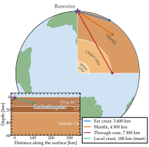
Geoneutrino geometry at Borexino. The geometry of a geoneutrino measurement at Borexino, at Gran Sasso, 1.4 km underground. A quarter of the Earth is cut away to expose the PREM layers of Figure The Earth’s density profile. Three chords reach production points beyond the local crust: in the far crust, 20 km deep and 3 400 km away; in the mantle, 1 000 km deep and 4 300 km away; and at the base of the mantle, 2 800 km deep and 7 300 km away, on a path through the outer core. The inset shows the local crust, to scale in distance and stretched in depth, with the crust layers of PREM and a production point 10 km deep and 100 km away. See notebook #28.
Geoneutrinos are the \(\bar{\nu}_e\) emitted in the decay chains of uranium-238 and thorium-232 inside the Earth [BILudhova+13]. Inverse beta decay can detect only those above 1.8 MeV. The most energetic geoneutrinos, from the uranium chain, reach 3.3 MeV, so the detectable spectrum spans 1.8–3.3 MeV. The sources are the crust and the mantle. Uranium and thorium are lithophile elements: they concentrate in silicate rock, and are expected to be absent from the metallic core. The core still enters the calculation, though, as the medium that neutrinos from the far side of the mantle cross. For a detector at or near the surface, the production points lie from a few km to a full Earth diameter away. As an example, we take Borexino [A+20c, A+09] as the detector, at Gran Sasso, 1.4 km underground.
Figure Geoneutrino geometry at Borexino shows the setup: four production points illustrate the kinds of path a geoneutrino takes to Borexino. One lies in the local crust, 10 km deep and 100 km away. One lies in the far crust, 20 km deep and 3 400 km away, on a path that dips into the upper mantle. One lies in the mantle, 1 000 km deep and 4 300 km away. The last lies at the base of the mantle, 2 800 km deep and 7 300 km away, on a path through the outer core.
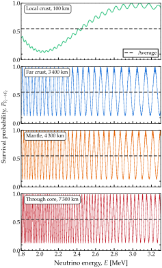
Geoneutrino survival against energy. Survival probability of \(\bar{\nu}_e\) geoneutrinos reaching Borexino, from the four production points of Figure Geoneutrino geometry at Borexino. In every panel, the fast oscillation of the pair split by \(\Delta m^2_{31}\) is resolved, riding as a fine ripple on the slower oscillation of the pair split by \(\Delta m^2_{21}\). This is visible only in the near-production case (top panel). In the three distant-production cases (bottom three panels), the line marks the phase average in vacuum, 0.548; matter raises it by 0.3–0.8%, less than the width of the line. Listing Geoneutrino survival against energy computes the four panels. See notebook #28.
Figure Geoneutrino survival against energy shows the survival probability against energy for these production points. Two oscillations appear: a slow one, from the pair of mass eigenstates split by \(\Delta m^2_{21}\), and a fast one, from the pairs split by \(\Delta m^2_{31}\). From the local crust, the slow oscillation completes less than one cycle across the window. From the three distant points, both complete tens to thousands of cycles, far more than a detector resolves in energy, so a measurement of a distant reservoir sees only the average probability. Within a few hundred kilometers of the detector, the slow oscillation does not average out across the window. For such nearby production points, the full probability must be used instead of the average; Figure Where the geoneutrino flux comes from uses it out to 331 km.
For the three distant production points, Figure Geoneutrino survival against energy marks the phase-averaged probability in vacuum, 0.548. Matter changes it little. The passage through the Earth is adiabatic: even the largest jump in electron density, at the core-mantle boundary, changes the mixing angle in matter by only about a percent at these energies, so the neutrino stays in the eigenstate in which it was produced. The average then depends only on the eigenstates at the two ends of the path [averaged limit on a varying profile, with \(P^{\rm cross}\) the identity; Phase-averaged probabilities]. At both ends, the matter potential is at most 2% of \(\Delta m^2_{21}/2E\), so those eigenstates are nearly the vacuum ones. As a result, matter raises the average by only 0.3–0.8%, less than the width of the line in Figure Geoneutrino survival against energy, and the vacuum value serves our calculation. The snippet below checks this along the mantle chord, with the density of PREM and the electron fraction of the mantle, using average=True (Asking for the averaged probability):
from magnus.earth import (
 distance_traveled_inside_earth as chord,
 earth_radial_distance_from_depth as radius,
 density_matter_func_prem as prem,
 Y_E_MANTLE_PREM)

osc = gd.load_nufit_params('NuFIT 6.1')

# The mantle chord: cosine of the zenith
# angle at the detector, and the depths of
# the production point and of Borexino [km]
c = -0.552
geo = dict(source_depth=1000.0,
           detector_depth=1.4)

# Length of the chord [km]
L = chord(c, **geo)

# Density along the chord [g/cm^3]: PREM,
# with its ocean layer replaced by rock
def rho(l):
    # Radius at distance l along the chord
    r = radius(c, l/gd.UNIT_KM, **geo)
    return prem(r,
                density_matter_ocean=2.65)

E = 2.5*gd.UNIT_MEV

# Phase-averaged survival probability in
# matter, at electron fraction of the mantle
P_m = oscprob.osc_prob_matter_std_potential(
 3, rho, E, L*gd.UNIT_KM, osc,
 average=True, nubar=True,
 nu_i=gd.NUE, nu_f=gd.NUE,
 electron_fraction=Y_E_MANTLE_PREM,
 density_matter_is_in_g_per_cm3=True)
# 0.551

# The same, in vacuum
P_v = oscprob.osc_prob_3nu_vacuum(E,
 L*gd.UNIT_KM, average=True, nubar=True,
 nu_i=gd.NUE, nu_f=gd.NUE)
# 0.548
Listing Geoneutrino survival against energy computes the panels of Figure Geoneutrino survival against energy with the Earth wrapper, osc_prob_3nu_earth. Each production point enters through its depth and the cosine of its zenith angle at the detector. Every chord crosses PREM boundaries—six on the far-crust chord, nine on the chord through the core—and the wrapper internally places a slab edge on each. Since Gran Sasso is a continental site, density_matter_ocean replaces the ocean layer of PREM with rock.
(When a source is buried, the wrapper automatically places it on the far side of the chord, where the chord first reaches the source depth. However, the local-crust production point, 10 km deep and 100 km away, lies instead on the near side: along its chord, a depth of 10 km is first reached about 1 100 km from the detector. To overcome this, the last call in Listing Geoneutrino survival against energy swaps the two ends of the path: it treats the detector as the source, 1.4 km deep, and the production point as the detector, 10 km deep, with the zenith angle measured at the production point. The result is unchanged, because the survival probability is the same along a path and along its reverse.)
Geoneutrino survival against energy. The four panels of Figure Geoneutrino survival against energy: the survival probability of a geoneutrino reaching Borexino from the far crust, the mantle, the base of the mantle, and the local crust, across the detectable window, on one energy grid fine enough to resolve the pair split by \(\Delta m^2_{31}\) on the longest chord. The call declares the PREM boundaries on each chord by itself. The ocean layer of PREM is replaced by rock. The local production point is run in reverse, from the detector. See notebook #28.
import numpy as np
import magnus.oscprob as oscprob
import magnus.globaldefs as gd

# Twelve energies per cycle of the pair split by
# Dm31^2 on the longest chord, 7,300 km
E = 1/np.linspace(1/1.8, 1/3.3, 22500)*gd.UNIT_MEV

# Borexino, 1.4 km underground.  A production point
# enters as its depth and the cosine of its zenith
# angle at the detector; the call declares the PREM
# boundaries on the chord by itself.  The oscillation
# parameters are the defaults, NuFIT 6.1.
points = {'far crust': (20.0, -0.272),    # 3,400 km
          'mantle': (1000.0, -0.552),     # 4,300 km
          'core': (2800.0, -0.872)}       # 7,300 km
P = {}
for name, (depth, costhz) in points.items():
    P[name] = oscprob.osc_prob_3nu_earth(E,
     costhz=costhz, source_depth=depth*gd.UNIT_KM,
     detector_depth=1.4*gd.UNIT_KM, nubar=True,
     nu_i=gd.NUE, nu_f=gd.NUE,
     density_matter_ocean=2.65)

# The local point, 10 km deep and 100 km away,
# run in reverse, from the detector (see text)
P['local'] = oscprob.osc_prob_3nu_earth(E,
 costhz=0.078, source_depth=1.4*gd.UNIT_KM,
 detector_depth=10.0*gd.UNIT_KM, nubar=True,
 nu_i=gd.NUE, nu_f=gd.NUE,
 density_matter_ocean=2.65)
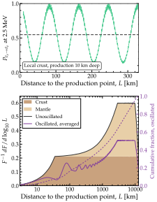
Where the geoneutrino flux comes from. Where the detectable geoneutrino flux at Borexino comes from and what oscillations leave of it. Top: the survival probability at 2.5 MeV against the distance to a production point 10 km deep, across the local crust, with the pair split by \(\Delta m^2_{31}\) resolved; the horizontal line is the phase average. Bottom: the distribution of the flux of Eq. (1) in the distance to the production point, per unit \(\log_{10} L\) and as a fraction of the total, for a spherically symmetric Earth with a 35-km crust holding 7 TW of radiogenic power, a mantle with the abundances of the geochemical model of Ref. [BILudhova+13], and no uranium or thorium in the core. The unoscillated curve has \(\langle P_{\bar\nu_e \to \bar\nu_e} \rangle = 1\). The oscillated curve folds in the survival probability averaged over the detectable window with equal weight in energy; its cumulative fraction is on the right axis. See notebook #28.
Figure Where the geoneutrino flux comes from shows how the detectable flux is distributed over the distance to the production point and how much of it survives the oscillations. A flux measurement weighs the curves of Figure Geoneutrino survival against energy by that distribution. The Earth model chosen for the figure is the simplest one that carries both reservoirs: a spherically symmetric crust 35 km thick holding 7 TW of radiogenic power at a thorium-to-uranium ratio of 4.5, a mantle with the abundances of the geochemical model of Ref. [BILudhova+13], no uranium or thorium in the core, and the density of PREM throughout. The flux at the detector, located at \(\mathbf{r}_{\rm det}\), is
where \(L \equiv \lvert \mathbf{r} - \mathbf{r}_{\rm det} \rvert\) and \(\varepsilon(\mathbf{r})\) is the number of detectable \(\bar{\nu}_e\) emitted per unit volume and time at position \(\mathbf{r}\), fixed by the density of PREM and the abundances above. The survival probability from that point, \(\langle P_{\bar\nu_e \to \bar\nu_e}(L) \rangle\), is the mean over the detectable window, 1.8–3.3 MeV. In spherical coordinates centered on the detector, \(d^3r = L^2 \, dL \, d\Omega\) and the \(L^2\) cancels: the production points between \(L\) and \(L + dL\) contribute \(dL / 4\pi\) times the emissivity integrated over the directions in which that shell lies inside the Earth. The lower panel of Figure Where the geoneutrino flux comes from shows this distribution per unit \(\log_{10} L\), normalized to the total flux without oscillations, so that the area under a curve between two distances is the share of the flux from between them. Without oscillations, the crust supplies 61% of the detectable flux, and the region within 350 km of the detector supplies 30%. Out to 331 km, the full probability must be used instead of the average.
The oscillated curve is the unoscillated one multiplied by \(\langle P_{\bar\nu_e \to \bar\nu_e}(L) \rangle\), the survival probability averaged over the detectable window. Up to 331 km, we compute the probability in full, at each distance on the grid, with the last call of Listing Geoneutrino survival against energy, and then average it over the window. Beyond 331 km, we use the average in vacuum instead, which differs from the full result by 0.01 at 331 km and by less farther out. The upper panel of Figure Where the geoneutrino flux comes from shows the full probability at 2.5 MeV: the slow oscillation has a period of 82 km, and the fast one, with a period of 2.5 km, appears as a ripple on it. Close to the detector, the window holds too few cycles of the slow oscillation to average it out, so the oscillated curve in the lower panel ripples out to a few hundred kilometers; farther out, it is smooth. Over the whole Earth, oscillations leave 54% of the detectable flux.
Both curves in the lower panel of Figure Where the geoneutrino flux comes from flatten at large distances, for a geometric reason. The production points at a distance \(L\) from the detector lie on a sphere of radius \(L\) centered on it. The part of this sphere at a distance between \(r\) and \(r + dr\) from the center of the Earth has area \(2 \pi L r \, dr / R_\oplus\). In Eq. (1), this area is divided by \(4 \pi L^2\), and on the logarithmic axis of the panel it is multiplied by \(L\), so the result does not depend on \(L\). Hence, a layer of the Earth contributes the same flux per decade of distance as long as the sphere reaches every depth of that layer. For the crust, this holds from 35 km out to a full Earth diameter; for the mantle, from about 2 900 to 9 900 km. The total stays flat over that range because the core, which holds no uranium or thorium in this model, adds nothing to it.
Neutrino tomography of the Sun
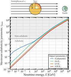
Adiabaticity along a solar chord. Top: the setup. An isotropic flux of \(\nu_e\) crosses the Sun and continues to Earth, where it may oscillate. The impact parameter \(b\) is marked on one ray. Bottom: Adiabaticity of a neutrino trajectory through the Sun against energy, computed with Magνs on the B16-GS98 solar density profile [VSV+17], tabulated up to the surface, for four impact parameters, each defining a chord through the Sun. The parameter \(\gamma_{\rm max}\) is the adiabaticity parameter of Adiabatic + Magnus hybrid strategy, evaluated at its maximum along the chord and over the three pairs of levels. See notebook #28.
Neutrinos made outside the Solar System arrive from all directions, so a share of them crosses the Sun on its way to Earth. At around 10 MeV, they come mainly from the diffuse supernova neutrino background; from TeV to PeV, they are part of the high-energy astrophysical flux. Below, we compute what that does to their oscillations, using the density profile of the B16-GS98 solar model [VSV+17] of Solar density profiles.
At the energies of this section, up to 1 PeV, a neutrino from a source outside the Solar System has traveled far enough for its oscillations to average out on the way (Figure The averaged flavor composition settles once the source is far enough.), so it reaches the Sun as an incoherent mixture of \(\nu_1\), \(\nu_2\), and \(\nu_3\). Therefore, the quantity to compute is the phase-averaged probability, propagated through the varying profile of the Sun as described in Phase-averaged probabilities. Where the passage is adiabatic, the neutrino stays in the instantaneous eigenstates of \(\mathbb{H}\); where it is not, Magνs crosses the region with a Magnus patch. Where every phase has averaged away, the result is averaged limit on a varying profile, with \(P^{\rm cross}\) the level-crossing matrix between the eigenbases at entry and exit. Both ends of the path lie in vacuum, where the eigenvectors of \(\mathbb{H}\) form the vacuum mixing matrix, so \(\mathbb{V}(l_0) = \mathbb{V}(l_1) = \mathbb{R}\) in averaged limit on a varying profile. If the passage is adiabatic, \(P^{\rm cross}\) is the identity, and averaged limit on a varying profile reduces to the vacuum averaged limit: the Sun leaves no trace. Whether the passage is adiabatic depends on the energy, through the adiabaticity parameter of Adiabatic + Magnus hybrid strategy.
This may seem at odds with the MSW effect, which changes solar neutrinos strongly (The Sun). The difference lies in where the path starts. A solar neutrino is born deep inside the Sun, at high density, as an eigenstate of \(\mathbb{H}\) in matter; an adiabatic passage outward turns it into a single vacuum mass eigenstate, which is a different state. A neutrino crossing the Sun from outside starts and ends in vacuum, so an adiabatic passage returns it to the same mass eigenstate it entered as.
Figure Adiabaticity along a solar chord shows how adiabatic the passage is, from MeV to PeV, at three flavors, for four impact parameters. The adiabaticity parameter \(\gamma_{jk}(l)\) of Adiabatic + Magnus hybrid strategy is defined for each pair of eigenvalues of \(\mathbb{H}\), 1-2, 1-3, and 2-3, at each point \(l\) of the path; it is large where the two eigenvalues come close. The figure plots its largest value along the chord and over the three pairs, \(\gamma_{\rm max}\). Where \(\gamma_{\rm max} > 1\), the passage is not adiabatic: somewhere along the chord, the neutrino moves between eigenstates of \(\mathbb{H}\). The adiabatic module of Magνs computes \(\gamma_{\rm max}\):
import numpy as np
import magnus.adiabatic as adiabatic
import magnus.hamiltonians as ham
import magnus.matter as matter
import magnus.globaldefs as gd
import magnus.solarmodels as solarmodels

osc = gd.load_nufit_params('NuFIT 6.1')
R = gd.SUN_RADIUS*gd.UNIT_KM
prof = solarmodels.electron_density_profile
ne_sun = prof('B16-GS98')
b = 0.3*R                # impact parameter
half = np.sqrt(R**2 - b**2)
E = 100.0*gd.UNIT_GEV
hv = ham.hamiltonian_3nu_vacuum(E, **osc)

def ne(l):
    """Electron density on the chord."""
    r = np.sqrt((l - half)**2 + b**2)
    return ne_sun(r)

def H(l):
    """Hamiltonian at l along the chord."""
    h = np.array(hv, dtype=complex)
    h[0, 0] += matter.VCC_func(l, ne)
    return h

info = {}
adiabatic.find_nonadiabatic_windows(
    H, 0.0, 2*half, n_probe=20000,
    info=info)
info['gamma_max']        # 13.7580
Here, ne_sun is the B16-GS98 table, interpolated in its logarithm, ne evaluates it along the chord, and hv is the vacuum Hamiltonian at this energy. The value shown is for a \(100\)-GeV neutrino crossing at an impact parameter of \(b = 0.3\,R_\odot\).
The parameter \(\gamma_{\rm max}\) grows with energy because the vacuum splitting \(\Delta m^2/2E\) shrinks while the matter potential stays fixed. The largest value comes from the 1-2 pair, near the point where its two eigenvalues come closest: the 1-2 resonance, where the matter potential equals \(\Delta m^2_{21}\cos 2\theta_{12}/2E\). This resonance occurs at a single radius in the Sun, set by the energy alone, so every chord reaches its \(\gamma_{\rm max}\) at that radius. As the energy grows, that density is reached further out: \(\gamma_{\rm max}\) sits at \(0.97\,R_\odot\) at \(100\) GeV, at \(0.990\,R_\odot\) at 1 TeV, and at \(0.998\,R_\odot\) at 100 TeV. By 1 PeV, it reaches \(5\times10^6\) on the diameter.
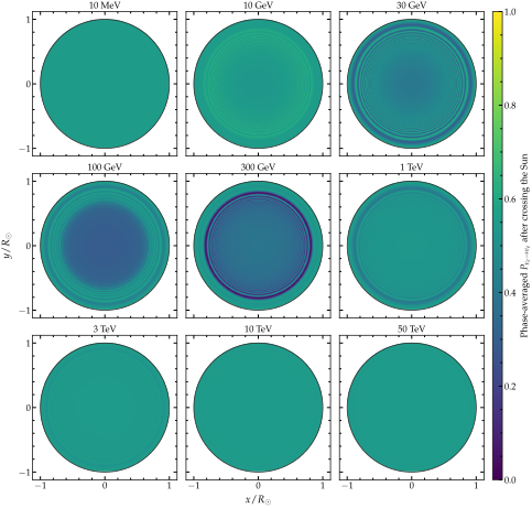
The Sun in the electron-neutrino channel. The Sun seen face-on in the \(\nu_e\) survival channel, computed with Magνs on the B16-GS98 solar density profile [VSV+17]. The line of sight runs into the page, so each point of the disk is an impact parameter and the neutrino crosses the whole Sun along it. The color is the phase-averaged \(P_{\nu_e \to \nu_e}\) at exit, for a relative energy spread of \(10%\), averaged over the area of each pixel. See notebook #28.
Figure The Sun in the electron-neutrino channel shows the averaged survival probability across the face of the Sun, at selected energies. The line of sight runs into the page, so each point in the disk fixes the impact parameter of one trajectory, along which the neutrino crosses the whole Sun. For one impact parameter, the probability is computed via
import magnus.oscprob as oscprob

# The chord above: b = 0.3 R_sun
P = oscprob.osc_prob_matter_std_potential(
    3, ne, E, 2*half, average=True,
    average_initial_state='decohered',
    osc_params=osc, L0=0.0, nu_i=gd.NUE,
    nu_f=gd.NUE,
    density_is_of_number_of_electrons=True)
P                        # 0.283618
Here, average=True returns the phase average along the chord, and average_initial_state='decohered' tells Magνs that the neutrino reaches the Sun decohered, i.e., as \(\nu_1\), \(\nu_2\), or \(\nu_3\) (Asking for the averaged probability). The default, 'flavor', would instead treat it as a \(\nu_e\) produced at the edge of the Sun, which keeps the interference between \(\nu_1\) and \(\nu_2\); their phase across the Sun is only about 1 rad at 100 GeV. The two choices give very different results on this chord:
kw = dict(
    osc_params=osc, L0=0.0, nu_i=gd.NUE,
    nu_f=gd.NUE, average=True,
    density_is_of_number_of_electrons=True)
f = oscprob.osc_prob_matter_std_potential
for start in ('flavor', 'decohered'):
    P = f(3, ne, E, 2*half, **kw,
          average_initial_state=start)
    print(start, P)  # 0.535944, 0.283618
A neutrino from a distant source arrives without that interference, which is why Figure The Sun in the electron-neutrino channel uses 'decohered'. Magνs computes the phase-averaged probability over the default relative energy spread of 10%, without sampling energies. Averaging a scan of probabilities over energy instead does not, in general, give the same result (Probability averaging). On this chord, a little interference survives the 10% spread, so the phase-averaged probability depends slightly on the spread, by about 0.01 per \(e\)-fold; Magνs issues a PhaseAveragingWarning saying so.
One phase survives the average: the matter phase, \(\int V_{\rm CC}\,dl\), which is \(8\,699\) rad across the solar diameter. Because it does not depend on energy, no energy spread averages it out. Each chord, however, crosses a different amount of matter, so the matter phase varies with the impact parameter. As \(b\) changes, the phase cycles through \(2\pi\) over and over, and \(P\) oscillates with it, drawing fine rings in the core of the disk. The rings are \(1.8\times10^{-4}\,R_\odot\) apart at \(b = 0.11\,R_\odot\) and \(5.1\times10^{-4}\,R_\odot\) apart at \(b = 0.3\,R_\odot\), and at 1 TeV they change \(P\) by up to about \(\pm 0.03\). The probability computed in the snippets above, \(P = 0.2836\) at \(b = 0.3\,R_\odot\), lies on one of these rings: as \(b\) moves by one ring spacing, \(5.1\times10^{-4}\,R_\odot\), around that value, \(P\) changes appreciably, from 0.282 to 0.308. These rings are far finer than any realistic experimental angular resolution, so an observation would average over many of them. Therefore, each pixel of Figure The Sun in the electron-neutrino channel is averaged over its area, which also keeps the rings from aliasing into false patterns. Each panel from 30 GeV to 3 TeV uses \(7\,791\) impact parameters. Most of them, \(6\,790\), lie inside \(b = 0.5\,R_\odot\), where the rings are densest.
At \(10\) MeV, the disk is uniform at \(\sum_i \lvert \mathbb{R}_{ei} \rvert^4 \approx 0.55\): the Sun is transparent, as \(P^{\rm cross} = \mathbb{1}\) requires. At intermediate energies, where Figure Adiabaticity along a solar chord shows the passage to be non-adiabatic, rings appear: there, the level-crossing probabilities depart from the identity. The phase average also keeps part of the interference between eigenstates that averaged limit on a varying profile drops, and this changes the depth of the rings: at 300 GeV, the deepest ring reaches \(P = 0.03\) at \(b = 0.81\,R_\odot\), against \(0.22\) from averaged limit on a varying profile. At higher energies, the deepest ring moves outward, to \(b = 0.88\,R_\odot\) at 1 TeV and \(0.91\,R_\odot\) at 10 and 50 TeV. At 50 TeV, the disk is uniform again, but for a different reason than at 10 MeV: inside the Sun, the matter potential dominates, so a \(\nu_e\) that enters the Sun leaves it as a \(\nu_e\), at every impact parameter, having only gained a phase, which does not affect the survival probability.
No neutrino telescope can resolve this structure. Super-Kamiokande has imaged the Sun in MeV neutrinos [H+06], but the image is blurred to about \(25^\circ\) at 10 MeV, because the recoil electron in neutrino-electron scattering follows the neutrino direction only loosely; the solar disk spans half a degree. At TeV energies, neutrino telescopes reconstruct muon tracks to within about \(1^\circ\) [A+20a], comparable to the size of the disk, and particle showers only to within \(10^\circ\)–\(40^\circ\) [A+19a]. The rings of Figure The Sun in the electron-neutrino channel, by contrast, are a few to a few tens of arcseconds wide. Moreover, at GeV energies, where the rings first appear, no astrophysical neutrino flux has been identified above the atmospheric background. Finally, both Figure Adiabaticity along a solar chord and Figure The Sun in the electron-neutrino channel include only oscillations: absorption in the Sun, which becomes important above about 100 GeV, is outside what Magνs models (limitations).
Astrophysical relativistic jet
Gamma-ray bursts are the relativistic jets that some massive stars launch as they collapse [MW99, Mes06, Pir04, Woo93]. Shells of plasma ejected by the central engine collide with one another along the jet [RM94]. Reference [PX94] first proposed these collisions as a source of neutrinos. Protons accelerated at those collisions can make TeV–PeV neutrinos [BBMW15, GHAM+04, HBW12, MN06, WB97]. The jet itself does not change their flavor composition: at the radii where the collisions happen, \(10^{13}\)–\(10^{15}\) cm, its density is around \(10^{-11}\) g cm\(^{-3}\), nine orders of magnitude below the density at which a TeV neutrino resonates; the phase that the jet matter adds to the evolution is below \(10^{-4}\). Matter effects arise only while the jet is still inside the star, in the choked jets that never break out and in the precursor phase of the jets that do [MMR07, RS10, SZ10, VSOOS15, XD15]. The neutrinos then cross the stellar envelope. Its density falls from about 0.3 g cm\(^{-3}\) at the head of the jet to zero at the surface, so every neutrino above about 50 GeV meets its 1-3 resonance somewhere along the way. At low energies, the crossing is adiabatic, and the neutrino leaves the star in a mass eigenstate; at high energies, it is not, and the neutrino keeps its flavor content. Therefore, the flavor ratios at Earth depend on the neutrino energy, in a way that reflects the density profile of the star [RS10, XD15].
As an example, we take a jet whose head is at \(r_0 = 6.3 \cdot 10^{10}\) cm, inside a blue supergiant of radius \(R_\star = 3 \cdot 10^{12}\) cm, with the hydrogen envelope of Refs. [MMR07, RS10], \(\rho(r) = 3.3 \cdot 10^{-6}\,(R_\star/r - 1)^3\) g cm\(^{-3}\), and an electron fraction of \(Y_e = 1\):
import numpy as np
import magnus.globaldefs as gd
import magnus.hamiltonians as ham
import magnus.oscprob as oscprob

OSC = gd.load_nufit_params('NuFIT 6.1')
CM = 1.0e-5*gd.UNIT_KM   # One cm in eV^-1
RSTAR = 3.0e12           # Star's radius, cm
R0 = 6.3e10              # Jet head, cm

def rho(l):
    """Density, g/cm3, at l in eV^-1."""
    return 3.3e-6*(RSTAR/(l/CM) - 1.0)**3
The density at the head is \(0.33\) g cm\(^{-3}\). The oscillation length there is set by the potential, \(2\pi/V_{\rm CC} \approx 5 \cdot 10^{9} {\rm cm} \approx 0.1 r_0\).
A neutrino born as \(\nu_\alpha\) at the jet head leaves the star in the state \(\mathbb{U}(R_\star, r_0)\,\lvert\nu_\alpha\rangle\), where \(\mathbb{U}(R_\star, r_0)\) is the evolution operator across the envelope. Its weight in the mass eigenstate \(\nu_i\) is
where \(\mathbb{V}(R_\star)\) is the vacuum mixing matrix. On its way to Earth, over a cosmological distance, the mass eigenstates lose coherence [RS10]. The probability at Earth is then
This is averaged limit on a varying profile, with the contribution of the star computed directly as \(w_{\alpha i}\) and the vacuum eigenbasis at detection.
The weights \(w_{\alpha i}\) depend on the relative phases of the flavor amplitudes at the surface of the star. The flavor probabilities, \(\lvert \mathbb{U}_{\beta\alpha}(R_\star, r_0) \rvert^2\), discard those phases, so the weights must be computed from the evolution operator. The scenario functions return the operator alongside the probabilities when called with return_evolution_operator=True. As usual, the refinement ladder chooses the slabs:
E = 1.0*gd.UNIT_TEV  # 1 TeV
# Evolve from the jet head (L0) to the
# surface (L); also return the operator
out = oscprob.osc_prob_matter_std_potential(
    3, rho, E, RSTAR*CM, OSC, L0=R0*CM,
    electron_fraction=1.0,  # hydrogen
    rtol=1.0e-6, atol=1.0e-6,
    density_matter_is_in_g_per_cm3=True,
    return_evolution_operator=True)
# Probabilities and evolution operator
P, U = out
Here, P holds the flavor probabilities at the surface of the star, and U is \(\mathbb{U}(R_\star, r_0)\) in the flavor basis.
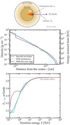
Jet neutrinos in a stellar envelope. Neutrinos from a relativistic jet inside a collapsing star. Top: the setup. Neutrinos are made at the head of the jet, at \(r_0 = 6.3 \cdot 10^{10}\) cm from the center, and leave the star at \(R_\star = 3 \cdot 10^{12}\) cm. Middle: matter density along their path, for a smooth envelope, the same envelope with turbulence overlaid, and the same envelope with a drop in density at the edge of the helium core. The right axis gives the energy whose 1-3 resonance lies at each density. Bottom: probability that a \(\nu_e\) produced at the jet head is detected as \(\nu_e\) at Earth, against its energy, for the three envelopes. See notebook #28.
From U, the weights and the probability at Earth follow:
# Vacuum mixing matrix, V(R_star)
hv = np.array(ham.hamiltonian_3nu_vacuum(
    E, **OSC), dtype=complex)
_, R = np.linalg.eigh(hv)
# Weights, w[i, alpha]
w = abs(R.conj().T @ U)**2
# Probability at Earth, P[beta, alpha]
P_earth = abs(R)**2 @ w
P_earth[gd.NUE, gd.NUE]    # 0.315
Without matter effects, the same calculation gives \(0.55\).
Figure Jet neutrinos in a stellar envelope shows this probability from 0.1 TeV to 10 PeV for three density envelopes. The first envelope is the smooth profile above. The second adds turbulence to it, as one realization of forty Kolmogorov modes with wavelengths from \(10^{10}\) to \(10^{12}\) cm and a root-mean-square amplitude of 20%. The third is model C of Refs. The third is model C of Ref. [MMR07], in which the density drops by a factor of five at the edge of the helium core, at \(10^{11}\) cm. The code receives this edge as a breakpoint. The neutrinos are made across a region about one oscillation length wide, so each curve averages over eight production points spread across that length. At the lowest energies, the resonance lies only a few oscillation lengths from the head. A single production point would then show an interference pattern, which the average removes.
Listing Jet neutrinos in a stellar envelope contains the calculation behind the figure. Each envelope takes well under a minute, over 161 energies and eight production points. At the requested tolerance of \(10^{-6}\), the ladder uses a few hundred slabs per energy at PeV energies and a few thousand at 0.1 TeV.
Jet neutrinos in a stellar envelope. Computing the data in Figure Jet neutrinos in a stellar envelope: the averaged \(\nu_e\) survival probability at Earth for neutrinos from a jet head at \(r_0\), through the three envelopes. Each call returns the evolution operator from the refinement ladder alongside the probabilities; the projection onto the vacuum mass states and the sum over them are averaged limit on a varying profile, with the eigenbasis at detection the vacuum one. The eight production points span one oscillation length at the jet head, \(4.9 \cdot 10^{9}\) cm. The turbulent envelope is one realization of forty Kolmogorov modes between \(10^{10}\) and \(10^{12}\) cm at 20% rms; the stepped one is model C of Refs. [MMR07], with the drop at the helium-core edge declared through t_breakpoints. See notebook #28.
import numpy as np
import magnus.globaldefs as gd
import magnus.hamiltonians as ham
import magnus.oscprob as oscprob

OSC = gd.load_nufit_params('NuFIT 6.1')
CM = 1.0e-5*gd.UNIT_KM               # One cm in eV^-1
RSTAR, R0, RHE = 3.0e12, 6.3e10, 1.0e11      # cm
E = np.geomspace(0.1, 1.0e4, 161)*gd.UNIT_TEV

# The three envelopes, g/cm3, r in cm
def smooth(r):
    return 3.3e-6*(RSTAR/r - 1.0)**3

rng = np.random.default_rng(7)
lam = np.geomspace(1.0e12, 1.0e10, 40)  # Modes, cm
k = 2*np.pi/lam
amp = k**(-1/3)                         # Kolmogorov
amp *= 0.20/np.sqrt(0.5*np.sum(amp**2)) # 20% rms
phi = rng.uniform(0.0, 2*np.pi, 40)
def turbulent(r):
    d = np.sum(amp*np.cos(k*r + phi))
    return smooth(r)*(1.0 + d)

def stepped(r):            # Mena et al., model C
    x = RSTAR/r - 1.0
    return 6.3e-6*(20.0*x**2.1 if r < RHE else x**2.5)

# Production points spread over one oscillation
# length at the jet head
r0s = R0 + 4.9e9*np.arange(8)/8.0

def p_earth(rho, **extra):
    """P at Earth, phase-averaged, and averaged
    over the production points."""
    P_out = np.zeros((len(E), 3, 3))
    for r0 in r0s:
        P, U = oscprob.osc_prob_matter_std_potential(
            3, lambda l: rho(l/CM), E, RSTAR*CM, OSC,
            L0=r0*CM, electron_fraction=1.0,
            density_matter_is_in_g_per_cm3=True,
            rtol=1.0e-6, atol=1.0e-6,
            return_evolution_operator=True, **extra)
        for i, e in enumerate(E):
            hv = np.array(ham.hamiltonian_3nu_vacuum(
                e, **OSC), dtype=complex)
            w, R = np.linalg.eigh(hv)
            content = abs(R.conj().T @ U[i])**2
            P_out[i] += abs(R)**2 @ content/len(r0s)
    return P_out

P_smooth = p_earth(smooth)
P_turb = p_earth(turbulent)
P_step = p_earth(stepped, t_breakpoints=[RHE*CM])
# Drawn: P_smooth[:, gd.NUE, gd.NUE], and the others
For the smooth envelope, the \(\nu_e\) survival probability at Earth rises with energy. At 0.1 TeV, a \(\nu_e\) leaves the star mostly as \(\nu_3\), the mass eigenstate with the smallest electron content, so it is rarely detected as \(\nu_e\). At 100 TeV, the probability reaches its vacuum value. The probability rises because the resonance crossing becomes less adiabatic as the energy grows. The resonance density falls as \(1/E\). Deep in the envelope, \(\rho \propto r^{-3}\), so the resonance moves outward as \(r_{\rm res} \propto E^{1/3}\). There, the density changes over a distance \(\rho/\lvert d\rho/dr \rvert = r_{\rm res}/3 \propto E^{1/3}\), while the oscillation length at the resonance grows as \(E\). Therefore, their ratio, which sets how adiabatic the crossing is, falls as \(E^{-2/3}\). At high energies, the crossing is non-adiabatic, and the neutrino keeps its flavor. At the PeV energies that IceCube detects, the star leaves the flavor content unchanged.
Turbulence shifts the probability by up to 0.05 below a few TeV. At these energies, the turbulent modes near the resonance have wavelengths comparable to the oscillation length (as in Turbulent matter profile). At the drop, the density falls by a factor of five within a small fraction of an oscillation length. Neutrinos between 0.1 and 0.55 TeV have their 1-3 resonance density inside the drop. They skip over their resonance, rather than crossing it gradually, so the crossing is non-adiabatic. This produces the plateau at about 0.36 in Figure Jet neutrinos in a stellar envelope, which extends to about 1 TeV. Above about 1.5 TeV, the resonance lies well outside the helium core, and the drop no longer matters: the stepped and smooth envelopes give the same probability to within 0.01.
Long-range interactions in the Sun
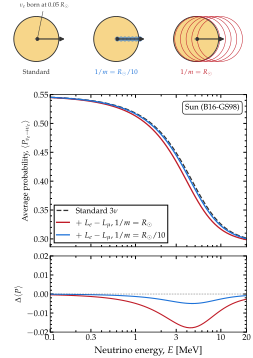
A long-range force in the Sun. Averaged \(\nu_e\) survival probability of solar neutrinos under a long-range \(L_e - L_\mu\) interaction sourced by solar electrons. Top: the electrons the neutrino feels at each mediator range. A \(\nu_e\) born at \(0.05\,R_\odot\) leaves along the drawn ray; the discs enclose the electrons within \(1/m\) of it. At \(1/m = R_\odot/10\), it feels a narrow tube of electrons; at \(1/m = R_\odot\), most of the Sun, even beyond the surface. The charged-current potential is local, so it has no disc. Middle: \(\langle P_{\nu_e \to \nu_e}\rangle\) against energy in the B16-GS98 model [VSV+17], without the new potential and with it at both ranges. The two ranges share one coupling, set so that the longer-ranged potential is \(0.1\,V_{\rm CC}\) at birth. The probability is read at \(20\,R_\odot\), where it has faded. Bottom: the difference from the standard case. See notebooks #19 and #28.
This example adds a new term to the Hamiltonian, one that Magνs does not ship. We write it as described in Building a new Hamiltonian from scratch, and average the probability as in the standard solar case of The Sun. The new term comes from gauging \(L_e - L_\mu\), the difference between the electron and muon lepton numbers, which is anomaly-free. Its gauge boson, \(Z'\), is a new light mediator [ABSS24, BA19a, HJLV91]. The charge \(L_e - L_\mu\) is \(+1\) for the electron and \(\nu_e\), \(-1\) for the muon and \(\nu_\mu\), and zero for every other field of the Standard Model. Therefore, the electrons of the Sun source a potential that \(\nu_e\) and \(\nu_\mu\) feel with opposite signs, and that \(\nu_\tau\) does not feel. The Hamiltonian is
where the first two terms are the standard vacuum and charged-current terms of Conventions, and the third is the new one.
Unlike \(V_{\rm CC}\), the new potential is non-local. Each electron sources a Yukawa potential around it, with a range set by the mass \(m\) of the \(Z'\). A neutrino at \(\mathbf{r}\) feels the electrons within about \(1/m\) of it:
where \(g^\prime\) is the new gauge coupling.
When the interaction range, \(1/m\), is larger than the body, the potential depends mainly on how many electrons the body holds, and only weakly on where they are [ABDN23, BA19a, WZ18]. When \(1/m\) is much shorter than the distance over which the density changes, only nearby electrons contribute, and \(V_{e\mu} \to g^{\prime 2} n_e(\mathbf{r})/m^2\). In this limit, the potential is local and proportional to \(V_{\rm CC}\), like a non-standard interaction with constant couplings [CGGM21]. Between the two limits, the potential depends on the shape of the density profile. For a spherical body, like the Sun, the angular integral can be done analytically. The potential then splits into the contributions of the electrons inside and outside radius \(r\):
where \({\rm shc}(x) \equiv \sinh(x)/x\). Both are running integrals over the density profile, so one pass over the table of a solar model gives the potential at every radius. For a massless mediator, \({\rm shc}\) and the exponentials tend to 1, and Eq. (4) becomes the Coulomb potential of the electrons. Notebook #19 derives Eq. (4) and checks it against the closed form for a uniform ball.
Figure A long-range force in the Sun shows the averaged \(\nu_e\) survival probability from 0.1 to 20 MeV. The density profile is from the B16-GS98 solar model [VSV+17]. The neutrino is born at \(0.05\,R_\odot\), near where \(^8\)B production peaks in that model. The figure compares the standard case with two mediator ranges, \(1/m = R_\odot\) and \(R_\odot/10\), corresponding to \(m \approx 3 \cdot 10^{-16}\) and \(3 \cdot 10^{-15}\) eV, respectively. Both ranges share one coupling. We fix it so that the longer-ranged potential is a tenth of \(V_{\rm CC}\) where the neutrino is born. The longer-ranged potential lowers the probability by up to 0.018, near 4 MeV. The shorter-ranged one lowers it by at most 0.005. Listing A long-range force in the Sun contains the calculation behind the figure.
At the same coupling, a longer range lets the neutrino feel more of the Sun’s electrons. Where the neutrino is born, the longer-ranged potential is \(0.10\,V_{\rm CC}\), about four times the shorter-ranged one, \(0.027\,V_{\rm CC}\). This difference at birth sets the difference between the two curves. The neutrino leaves the Sun adiabatically, so its averaged probability depends only on the Hamiltonian where it is born and where it is detected.
Along the path, both new potentials fall more slowly than \(V_{\rm CC}\). The electron density of the Sun falls by about five orders of magnitude from the center to \(0.98\,R_\odot\), and \(V_{\rm CC}\) falls with it. In contrast, \(V_{e\mu}\) is an integral over the electrons within about \(1/m\), which for the longer range include those of the dense core. In Listing A long-range force in the Sun, the ratio \(V_{e\mu}/V_{\rm CC}\) at half a solar radius is
half = np.searchsorted(r, 0.5*R_SUN)
v_emu[1.0][half]/vcc[half]     # 2.39
v_emu[0.1][half]/vcc[half]     # 0.098
At \(0.98\,R_\odot\), the two ratios are about 700 and 1.2. The top panel of Figure A long-range force in the Sun illustrates this. With \(1/m = R_\odot\), the neutrino feels most of the Sun wherever it is, and the potential extends beyond the surface. We read out the probability at \(20\,R_\odot\) away from the solar center, where the new potential has faded.
In Listing A long-range force in the Sun, the Hamiltonian accepts an array of positions, so the engine can evaluate it at many positions in one call (Performance). The averaged probability comes from osc_prob_energy_baseline with average=True. The standard case uses the same call, with \(V_{e\mu} = 0\). At 10 MeV,
i = np.argmin(abs(Es - 10.0*gd.UNIT_MEV))
P_std[i]                      # 0.325
P_lri[1.0][i], P_lri[0.1][i]  # 0.317, 0.323
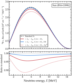
The \(^8\)B neutrino flux at Earth under a long-range force. Top: flux of \(\nu_e\) from \(^8\)B decay at Earth, against energy, for the standard case and for the two mediator ranges of Figure A long-range force in the Sun, with the same coupling. The dotted curve has \(1/m = R_\odot\) and a coupling \(g^{\prime 2}\) three times larger. The fluxes are the \(^8\)B spectrum of Ref. [WFRS06] times the total flux of the B16-GS98 model, \(5.46 \cdot 10^6\) cm-2 s-1 [VSV+17], times the survival probability averaged over where \(^8\)B neutrinos are made in the model. Bottom: each case divided by the standard one. See notebook #28.
Figure The 8B neutrino flux at Earth under a long-range force shows the flux of \(\nu_e\) from \(^8\)B decay at Earth, from 1 to 15 MeV. Since \(^8\)B neutrinos are produced over a range of radii, 80% of them between \(0.025\,R_\odot\) and \(0.081\,R_\odot\) in the B16-GS98 model, we average the survival probability over the production distribution:
where \(\Phi_{^8{\rm B}} = 5.46 \cdot 10^6\) cm-2 s-1 is the total flux of the model [VSV+17], \(\lambda(E)\) is the \(^8\)B spectrum normalized to unity [WFRS06], \(f(r)\) is the radial distribution of production, normalized to unity, and \(\langle P_{\nu_e \to \nu_e}(E; r) \rangle\) is the averaged survival probability of a neutrino born at radius \(r\). We evaluate the integral on 28 radii between \(0.005\,R_\odot\) and \(0.14\,R_\odot\), which contain 99.9% of production.
(We compute \(f(r)\) from the temperature, density, and composition of B16-GS98, as the rate of \(^7\)Be(p, γ) \(^8\)B. In this rate, \(^7\)Be is in equilibrium between its production by \(^3\)He(α, γ) \(^7\)Be and its destruction by electron and proton capture, with the reaction rates of Ref. [A+11]. To test this calculation, we apply it to an older solar model, BS2005-AGS,OP, whose \(^8\)B production distribution is published [BSB05]. The two distributions agree within 1% of the peak. Notebook #28 contains the calculations.)
Extending Listing A long-range force in the Sun, Eq. (5) for \(1/m = R_\odot\) is
# Birth radii, weighted by where 8B is made
r_b = np.linspace(0.005, 0.14, 28)*R_SUN
w = f(r_b)*np.gradient(r_b)
w = w/w.sum()
# Average over them, then scale by the 8B
# spectrum and total flux, cm^-2 s^-1 MeV^-1
P = sum(wk*averaged(v_emu[1.0], rk)
        for rk, wk in zip(r_b, w))
flux = 5.46e6*spectrum(Es)*P
where f and spectrum interpolate \(f(r)\) and \(\lambda(E)\). The longer-ranged potential lowers the flux by up to 4.5%, near 5 MeV, and by 3.6% in total above 1 MeV. The shorter-ranged one lowers it by at most 1.3%. Tripling \(g^{\prime 2}\) for \(1/m = R_\odot\) lowers it by up to 11%, near 4.5 MeV.
A long-range force in the Sun. Computing the data in Figure A long-range force in the Sun. The electron density comes from the B16-GS98 table [VSV+17], continued past the surface. The potential \(V_{e\mu}\) is Eq. (4) on that profile. The vacuum and matter terms come from the shipped builders; only the new term is written here. The neutrino is born at \(0.05\,R_\odot\), and the averaged probability is read out at \(20\,R_\odot\). See notebooks #19 and #28.
import numpy as np
import magnus.globaldefs as gd
import magnus.hamiltonians as ham
import magnus.matter as matter
import magnus.oscprob as oscprob
import magnus.solarmodels as solarmodels

osc = gd.load_nufit_params('NuFIT 6.1')

# The B16-GS98 model that ships with Magnus,
# on its tabulated radii and on to 20 R_sun
model = 'B16-GS98'
tab = solarmodels.load_solar_model(model)
r_tab = tab['r_over_r_sun']*gd.SUN_RADIUS*gd.UNIT_KM
R_SUN = r_tab[-1]                   # The surface
R0, R_END = 0.05*R_SUN, 20.0*R_SUN  # Birth, readout
r = np.concatenate([r_tab, np.geomspace(
    1.002*R_SUN, R_END, 800)])
ne_func = solarmodels.electron_density_profile(model)
n_e = ne_func(r)                    # Fades past R_SUN
per_ne = matter.VCC_func(0.0, lambda l: 1.0)
vcc = per_ne*n_e

def vcc_sun(l):
    """V_CC at l."""
    return per_ne*ne_func(l)

def cumulative(y, x):
    """Running trapezoidal integral, zero at x[0]."""
    steps = 0.5*(y[1:] + y[:-1])*np.diff(x)
    return np.concatenate([[0.0], np.cumsum(steps)])

def shc(x):
    """sinh(x)/x, equal to 1 at the origin."""
    x = np.asarray(x, dtype=float)
    return np.divide(np.sinh(x), x, out=np.ones_like(x),
                     where=(x != 0.0))

def long_range_potential(r, n_e, m):
    """V_emu(r)/g'^2 for a spherical n_e."""
    I_in = cumulative(r**2*n_e*shc(m*r), r)
    I_out = cumulative(r*n_e*np.exp(-m*r), r)
    I_out = I_out[-1] - I_out      # From r outward
    r_safe = np.where(r > 0.0, r, 1.0e-30)
    return np.exp(-m*r)*I_in/r_safe + shc(m*r)*I_out

# Two mediator ranges, one coupling: g'^2 makes V_emu
# a tenth of V_CC at R0 when 1/m = R_sun
v_emu = {}
for frac in (1.0, 0.1):            # 1/m in R_sun
    v_emu[frac] = long_range_potential(
        r, n_e, 1.0/(frac*R_SUN))
g2 = 0.1*vcc_sun(R0)/np.interp(R0, r, v_emu[1.0])
v_emu = {frac: g2*v for frac, v in v_emu.items()}

# The standard part from the shipped builders; the
# new term is the only line written here
h_vac = ham.\
    hamiltonian_3nu_vacuum_energy_independent(**osc)
q = np.diag([1.0, -1.0, 0.0])     # L_e-L_mu charges

def H_lri(v):
    """H(E, l) of the text, with V_emu = v."""
    def H(E, l):
        h_matt = ham.hamiltonian_3nu_matter_td(
            l, vcc_sun)
        return (h_vac/E + h_matt
                + np.interp(l, r, v)[..., None, None]*q)
    return H

Es = np.logspace(-1.0, np.log10(20.0), 70)*gd.UNIT_MEV

def averaged(v, r0=R0):
    """<P_ee> from r0 to R_END, per E."""
    return oscprob.osc_prob_energy_baseline(
        H_lri(v), Es, R_END, r0, nu_i=gd.NUE,
        nu_f=gd.NUE, average=True)

P_std = averaged(0.0*vcc)
P_lri = {frac: averaged(v_emu[frac]) for frac in v_emu}
Turbulent matter profile
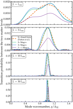
Turbulence: numerical against theory. Transition probability between two matter levels, against the wavenumber \(q\) of a single density mode of amplitude \(C = 0.03\), for a 5-GeV neutrino crossing a region of mean density \(\rho_0 = 4\) g cm\(^{-3}\). The levels are those of the mean density, between which no transition occurs without the mode. The panels are region lengths of \(1\), \(3\), \(10\), and \(30\,L_{\rm osc}\), with \(L_{\rm osc} = 2\pi/\Delta_{32} = 11\,030\) km. The closed form of Refs. [PKM14, PKM15], Eq. (6), is evaluated for the two-flavor reduction of the 1–3 sector. Magνs is run at two, three, and four flavors, the last with \(\sin^2\theta_{14} = \sin^2\theta_{24} = 0.10\) and \(\Delta m^2_{41} = 1\) eV\(^2\). See notebook #28.
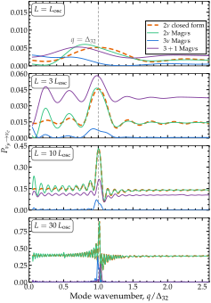
The same mode in the flavor channel. Probability \(P_{\nu_\mu \to \nu_e}\) for the same neutrino, medium, mode, and region lengths as Figure Turbulence: numerical against theory, at two, three, and four flavors. The line labeled \(q = \Delta_{32}\) marks the mode that matches the three-flavor gap; the two- and four-flavor gaps lie 2% and 3.5% above it. The curves sit at different heights because, even without the mode, the three flavor counts give different probabilities. The closed-form curve is Eq. (8), for the same two-flavor system as in Figure Turbulence: numerical against theory. See notebook #28.
Matter behind a supernova shock does not settle, because convection keeps stirring it. Its density fluctuates about its mean by tens of percent, on length scales from the size of the star to far below it [FLMM06, LQFB95, PKM14, PKM15]. Therefore, the density along the path of an escaping neutrino has two components: a smooth profile that decreases with radius, and random fluctuations on top of it. The fluctuations can be decomposed into Fourier modes, each a periodic density variation of wavenumber \(q\). A mode moves neutrinos between two eigenstates of \(\mathbb{H}\) when \(q\) matches the gap between their eigenvalues, \(\Delta_{jk} = \lambda_j - \lambda_k\). This is the parametric resonance of Methodology.
References [PKM14, PKM15] solved this problem in closed form. They treated the random component as a perturbation of the regular one and kept only its resonant term. For a density mode \(\rho(l) = \rho_0 \left[1 + C \cos(q l)\right]\), with \(\rho_0\) the mean density and \(C\) the relative amplitude of the mode, they obtained a Rabi formula for the transition between the two levels,
where \(L\) is the length of the turbulent region and \(p \equiv \tfrac{1}{2} (\Delta_{jk} - q )\) is the detuning of the mode from the gap. The coupling the mode induces between the levels is \(\kappa \equiv \tfrac{1}{2} C V_{\rm CC} \lvert U^m_{ej} U^m_{ek}\rvert\), with \(U^m\) the mixing matrix in matter at \(\rho_0\). On resonance, where \(q = \Delta_{jk}\), the probability is \(\sin^2(\kappa L)\). Complete conversion requires a region of length \(\pi/(2\kappa)\), which grows as \(C\) shrinks.
As an example, we consider a 5-GeV neutrino crossing a region of mean density \(\rho_0 = 4\) g cm\(^{-3}\) that carries one mode of amplitude \(C = 0.03\):
import numpy as np
import magnus.globaldefs as gd
import magnus.matter as matter
import magnus.hamiltonians as ham

OSC = gd.load_nufit_params('NuFIT 6.1')
E = 5.0*gd.UNIT_GEV    # Neutrino energy
RHO0 = 4.0             # Mean density, g/cm3
C = 0.03               # Mode amplitude

def one_mode(q):
    """Density along the ray: the mean, plus
    one mode of wavenumber q."""
    def rho(l):
        x = np.asarray(l, dtype=float)
        return RHO0*(1.0 + C*np.cos(q*x))
    return rho
The gaps of \(\mathbb{H}\) at \(\rho_0\) set the range of \(q\) to scan:
# n_e and V_CC of the smooth medium
ne0 = matter.num_density_e_func(
    0.0, lambda l: RHO0,
    density_matter_is_in_g_per_cm3=True)
V0 = matter.VCC_func(0.0, lambda l: ne0)

# H at the mean density: vacuum plus matter
H0 = np.array(ham.hamiltonian_3nu_vacuum(
    E, **OSC), dtype=complex)
H0 += ham.hamiltonian_3nu_matter(V0)

# Eigenvalues w, matter eigenvectors Vm, and
# the gap the mode has to match
w, Vm = np.linalg.eigh(H0)
d32 = abs(w[2] - w[1])
LOSC = 2*np.pi/d32     # 11 030 km

# Coupling of levels 2 and 3, and the length
# of complete conversion, in units of LOSC
kap = 0.5*C*V0*abs(Vm[0, 1]*Vm[0, 2])
np.pi/(2*kap)/LOSC     # 37.4
The mode that matches \(\Delta_{32}\) has wavelength \(L_{\rm osc} \equiv 2\pi/\Delta_{32} = 11\,030\) km, the oscillation length of levels 2 and 3. Complete conversion between them takes \(37\,L_{\rm osc}\). Only these two levels carry appreciable electron flavor, since \(\lvert U^m_{e1} \rvert^2 = 5.5 \times 10^{-4}\). Hence, the modes that match the other two gaps, \(\Delta_{21}\) and \(\Delta_{31}\), couple their levels about 15 and 40 times more weakly.
Magνs computes the same transition probability without the approximations behind Eq. (6), from the evolution operator \(\mathbb{U}\) (The Hamiltonian and the probability). Written in the basis of the eigenstates at \(\rho_0\), its element \(\lvert [\mathbb{U}]_{jk} \rvert^2\) is the probability of a transition from level \(k\) to level \(j\). In a medium of constant density, \(\mathbb{H}\) is diagonal in that basis at every point. Each level then evolves on its own, and \([\mathbb{U}]_{jk}\) vanishes for \(j \neq k\). The mode adds \(C V_{\rm CC} \cos(ql)\, U^{m*}_{ej} U^m_{ek}\) to each element of \(\mathbb{H}\) in that basis. The off-diagonal elements mix the levels as the neutrino advances, and \(\lvert [\mathbb{U}]_{jk} \rvert^2\) measures that mixing over the whole region. The diagonal elements raise and lower the levels with the density. Magνs returns \(\mathbb{U}\) in the flavor basis; rotating it to the matter basis takes one line:
from magnus.oscprob import (
  compute_evolution_operator_multiple_slabs
  as chain)

L = LOSC             # The region, one L_osc
rho = one_mode(d32)  # Mode tuned to the gap

def H(l):
    """H at position l, with the mode on."""
    h = np.array(ham.hamiltonian_3nu_vacuum(
        E, **OSC), dtype=complex)
    # V_CC follows the density
    return h + ham.hamiltonian_3nu_matter(
        V0*rho(l)/RHO0)

# One operator per slab, from 9 nodes at
# Magnus order 6
edges = np.linspace(0.0, L, 501)
slabs = np.stack([edges[:-1], edges[1:]], 1)
Us = chain(H, slabs, 9, 6)

# Ordered product, earliest slab first
U = Us[0]
for u in Us[1:]:
    U = u @ U

# Rotate to the matter basis, then read the
# transition between levels 2 and 3
P32 = abs((Vm.conj().T @ U @ Vm)[2, 1])**2
P32                    # 0.001758
Figure Turbulence: numerical against theory shows this probability against \(q\) for four lengths of the region, computed with Magνs and with Eq. (6). We evaluate the closed form for the two-flavor 1–3 sector, the system for which it was derived. The closed form relies on the rotating-wave approximation, which neglects a rapidly oscillating part of the coupling; that part averages out only over many oscillation lengths. Hence, it is accurate only in long regions: it differs from the two-flavor Magνs result by 28% of the peak at \(L = L_{\rm osc}\), but by only 0.4% at \(L = 30\,L_{\rm osc}\). The resonance narrows as the region lengthens, because a longer region requires a closer match between \(q\) and the gap. Adding flavors changes the eigenvalues of \(\mathbb{H}\), and with them the gap that the mode must match. Hence, the resonance lies at \(q/\Delta_{32} = 1.020\), \(1\), and \(1.035\) for two, three, and four flavors. The sterile state also draws 10% of the electron flavor into the fourth level. This lowers \(\lvert U^m_{e2} U^m_{e3} \rvert\) from 0.33 to 0.25, so the coupling \(\kappa\) is weaker and the four-flavor peak is lower.
Figure The same mode in the flavor channel shows the flavor probability \(P_{\nu_\mu \to \nu_e}\) for the same sweep, computed via
import magnus.oscprob as oscprob

kw = dict(
    nu_i=gd.NUMU, nu_f=gd.NUE,
    density_matter_is_in_g_per_cm3=True)

# Two flavors: the 1-3 sector
OSC2 = dict(sth=OSC['s13'], Dm2=OSC['D31'])
P2 = oscprob.osc_prob_matter_std_potential(
    2, one_mode(d32), E, L, OSC2, **kw)

# Three flavors
P3 = oscprob.osc_prob_matter_std_potential(
    3, one_mode(d32), E, L, OSC, **kw)

# The same call with a sterile state added
OSC4 = dict(OSC, s14=np.sqrt(0.10), D41=1.0,
            s24=np.sqrt(0.10), s34=0.0,
            d14=0.0, d24=0.0)
P4 = oscprob.osc_prob_matter_std_potential(
    4, one_mode(d32), E, L, OSC4, **kw)
From \(10\,L_{\rm osc}\) on, the probability changes most near \(q = \Delta_{32}\). This is the resonance of Figure Turbulence: numerical against theory, now seen in the flavor channel; as before, it narrows as the region lengthens. In shorter regions, modes with \(q < \Delta_{32}\) change the probability by a comparable or larger amount; we explain why below. For \(q > \Delta_{32}\), the curves return to their values in the smooth medium. The three-flavor curve shows no resonance at the other two gaps, \(\Delta_{21} = 1.26\,\Delta_{32}\) and \(\Delta_{31} = 2.26\,\Delta_{32}\), because the modes that match them couple their levels only weakly.
Figure The same mode in the flavor channel also shows a flavor probability computed from the closed form. Eq. (6) follows from the propagator of the two-level system in the rotating-wave approximation [PKM14, PKM15]. Rotated to the flavor basis, it reproduces the resonance computed by Magνs, but not the effect of modes slower than the gap. In the matter basis at \(\rho_0\), the propagator is
where \(\bar\lambda = \tfrac{1}{2}(\lambda_1 + \lambda_2)\) is the mean of the two levels, \(p = \tfrac{1}{2}(\lambda_2 - \lambda_1 - q)\) is the detuning, and \(\kappa_c = \tfrac{1}{2} C V_{\rm CC}\, U^{m*}_{e1} U^m_{e2}\) is the coupling, with \(\lvert \kappa_c \rvert = \kappa\). The matrix in the exponent is the Hamiltonian in a frame that rotates with the mode. In that frame, the Hamiltonian does not depend on position, so the propagator is a single matrix exponential. The diagonal prefactor transforms the result back to the matter basis. In the flavor basis, the probability is
Of the terms that the mode adds to \(\mathbb{H}\), the rotating-wave approximation keeps only the off-diagonal part that oscillates in step with the transition between the two levels. It discards the rest, including the diagonal terms, which shift the levels up and down with the density. Below the resonance, the off-diagonal terms drive no transition, as Figure Turbulence: numerical against theory shows. The diagonal terms still matter there: the levels follow the slowly varying density, which changes the phases they accumulate and, with them, \(P_{\nu_\mu \to \nu_e}\). Eq. (7) lacks these terms, so its curve stays at the value for the smooth medium.