A supernova shock front
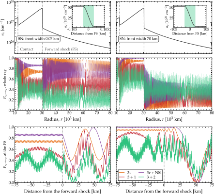
A supernova shock front. Electron density along a supernova ray, and the survival probability of a 15-MeV \(\nu_e\) along it. Top: the density from \(10^{4}\) to \(8 \cdot 10^{4}\) km, with the contact discontinuity at 12,348 km, where the density jumps by a factor of 2.5, and the forward shock at 30,323 km, where it jumps tenfold. The columns differ only in the width of both fronts: 0.07 km on the left, 70 km on the right. The insets enlarge the forward shock, with its width shaded. Center: the probability along the ray, computed with Magνs at :math:`rtol = 10^{-8}` for four Hamiltonians. The ray holds thousands of oscillation lengths of the pair split by \(\Delta m^2_{31}\), so the panel shows the envelope of the oscillation. The two columns agree bitwise up to the contact discontinuity. Bottom: a window of \(\pm\)75 km around the forward shock, where the oscillation is resolved. Two flavors are not drawn: with \(\Delta m^2_{21}\) alone, the probability stays above 0.95. The profile follows Refs. [FLMM03, SF02], with the radii of a simulation snapshot [KK15]. Listing Through a supernova shock front computes the left column. See notebooks #14 and #28.
Figure A supernova shock front shows the survival probability of a 15-MeV \(\nu_e\) along a supernova ray crossed by a shock, for two widths of the shock fronts, 0.07 and 70 km. The forward shock is the blast wave of the explosion. It propagates outward through an envelope whose density falls as \(r^{-2.4}\), and compresses the matter behind it tenfold. Behind it lies the contact discontinuity, which separates the shocked envelope from the ejecta; across it, the density drops by a factor of 2.5, while the pressure is continuous. Therefore, an outgoing neutrino crosses two density jumps: first the contact discontinuity, then the forward shock. Between them lies the shocked shell, thinned by a rarefaction. Because a shock alters the adiabaticity of the level crossings, it leaves a signature in the neutrino signal [FLMM03, SF02].
At three flavors, only the pair of eigenstates split by \(\Delta m^2_{31}\) is affected. The resonance density of the pair split by \(\Delta m^2_{21}\) is 7 times lower than the lowest density on the ray, so that pair never reaches resonance; accordingly, the two-flavor survival probability stays above 0.95. At 15 MeV, the resonance density of the pair split by \(\Delta m^2_{31}\) lies between the densities on either side of the forward shock, so the resonance is crossed at the front, where the oscillation length is about 50 km.
The 0.07-km front is crossed suddenly, before the state can follow the eigenstates. Across the 70-km front, which is comparable to the oscillation length, the state partly follows them. Therefore, beyond the forward shock, the mean survival probability at three flavors is 0.84 for the sharp fronts and 0.20 for the wide ones. The other Hamiltonians shift by different amounts; for 3+2, the shift is reversed, from 0.22 to 0.38.
Listing Through a supernova shock front computes the curves of the left column. It declares both fronts through t_breakpoints, as the positions where each begins and ends, so that every level of the refinement places slab edges there. Without the breakpoints, a 0.07-km front falls inside a slab at every level, and a slab that contains a jump degrades the quadrature regardless of the number of slabs. The three-flavor scan is then wrong beyond the forward shock by up to 0.25, and Magνs warns:
P = oscprob.osc_prob_matter_std_potential(
 3, ne_shock, 15.0*gd.UNIT_MEV, Ls, osc,
 L0=10000.0*gd.UNIT_KM, rtol=1.0e-8,
 atol=1.0e-10, nu_i=gd.NUE, nu_f=gd.NUE,
 density_is_of_number_of_electrons=True)
# UnmarkedDiscontinuityWarning: the
# Hamiltonian is discontinuous at the scale
# of the grid this scan builds, and no
# t_breakpoints were given.  A slab
# straddling a density jump degrades the
# quadrature no matter how many slabs are
# used; pass t_breakpoints at the
# discontinuities.
With or without breakpoints, the scan also raises two tolerance warnings, because at rtol \(= 10^{-8}\) the refinement reaches its cap of 20 000 slabs before certifying the result. With the fronts declared, the cap is immaterial: raising it tenfold changes the curve by less than \(10^{-5}\), well below the resolution of Figure A supernova shock front. The scans go to the cumulative engine, as the last line of the three-flavor call confirms; declared breakpoints would keep the hybrid engine of Adiabatic + Magnus hybrid strategy out in any case. Notebook #14 checks the result against an independent integration, and Against other codes measures the cost of the front width.
Through a supernova shock front. The four curves of the left column of Figure A supernova shock front: for each Hamiltonian, a scan of 4 000 baselines along the ray at one energy, with both fronts declared. t_breakpoints names the positions where each front begins and ends, and the refinement puts slab edges there at every level. ne_shock is the electron density of Figure A supernova shock front, the profile of notebook #14, with \(Y_e = 1/2\) and the normalization the model was defined with: the mean free-nucleon mass and the gram as converted before 1.2.0. See notebook #14.
import numpy as np
import magnus.oscprob as oscprob
import magnus.globaldefs as gd

osc = gd.load_nufit_params('NuFIT 6.1')

# The model's normalization: the mean free-nucleon
# mass, and the gram as converted before 1.2.0
MEAN_NUCLEON = (0.5*(gd.MASS_PROTON + gd.MASS_NEUTRON)
                *1.783e-33/gd.CONV_EV_TO_G)

# The ray: an r^-2.4 envelope, compressed tenfold
# behind the forward shock (thinned by a
# rarefaction) and 2.5 times more inside the contact
# discontinuity.  Each front is a smooth step of
# width w_km
R_CD, R_FS, w_km = 12348.0, 30323.0, 0.07   # km

def step(r, r0):
    u = np.clip((r0 + w_km/2 - r)/w_km, 0.0, 1.0)
    return u*u*(3.0 - 2.0*u)

def ne_shock(l):
    r = np.asarray(l)/gd.UNIT_KM
    u = np.clip(1.0 - r/R_FS, 0.0, 1.0)
    rare = np.exp((0.28 - 0.69*np.log(R_FS))
                  *np.arcsin(u)**1.1)
    rho = (1.0e14*r**-2.4                  # g/cm^3
           *(1.0 + step(r, R_FS)*(10.0*rare - 1.0))
           *(1.0 + 1.5*step(r, R_CD)))
    # Y_e = 1/2, with the model's own normalization
    return (rho*gd.UNIT_G_PER_CM3
            /MEAN_NUCLEON*0.5)

# Declare where each front begins and ends
w = w_km*gd.UNIT_KM
edges = [r*gd.UNIT_KM + s*w/2 for r in (R_CD, R_FS)
         for s in (-1.0, 1.0)]

# 4000 baselines from 10,200 to 80,000 km, at one
# energy: the cumulative engine answers
Ls = np.linspace(10200.0, 80000.0, 4000)*gd.UNIT_KM
run = dict(L0=10000.0*gd.UNIT_KM, t_breakpoints=edges,
 rtol=1.0e-8, atol=1.0e-10, nu_i=gd.NUE, nu_f=gd.NUE,
 density_is_of_number_of_electrons=True)
E = 15.0*gd.UNIT_MEV

# Standard three-flavor oscillations
info = {}
P3 = oscprob.osc_prob_matter_std_potential(
 3, ne_shock, E, Ls, osc, strategy_info=info, **run)
info['engine']   # 'cumulative'

# The same, with non-standard interactions
eps = dict(eps_ee=0.10, eps_em=0.05, eps_et=0.0,
 eps_mm=0.0, eps_mt=0.03, eps_tt=0.0)
P3_nsi = oscprob.osc_prob_matter_nsi(
 3, ne_shock, E, Ls, osc, eps, **run)

# One and two sterile states
osc4 = dict(osc, s14=0.10**0.5, s24=0.10**0.5,
 s34=0.0, D41=1.0, d14=0.0, d24=0.0)
P4 = oscprob.osc_prob_matter_std_potential(
 4, ne_shock, E, Ls, osc4, **run)
osc5 = dict(osc4, s15=0.06**0.5, s25=0.06**0.5,
 s35=0.0, D51=1.7, d15=0.0, d35=0.0)
P5 = oscprob.osc_prob_matter_std_potential(
 5, ne_shock, E, Ls, osc5, **run)
A detector measures the survival probability averaged over its energy resolution. The average washes out two phases: the one accumulated after the forward shock, thousands of cycles by the end of the ray at 15 MeV and far more on the way to Earth, and the one accumulated between the two fronts. The latter arises because the neutrino can change eigenstate at either front, so the paths through the shocked shell interfere; the interference completes a cycle every 15 keV. On the Sun, the averaged limit on a varying profile required only the eigenbases at the ends of the ray, because the passage was adiabatic and \(P^{\rm cross}\) was the identity. Here, the fronts are crossed suddenly, \(P^{\rm cross}\) depends on their width, and the amplitudes of the two paths add before the modulus is taken.
Without declared fronts, average=True resolves the 70-km fronts: it returns 0.37, against \(0.35 \pm 0.04\) with the fronts declared. It cannot resolve the 0.07-km fronts: it treats them as smooth, returns 0.04, close to the few percent obtained without a shock (Figure The shock signature against energy), instead of 0.56, and raises UnmarkedDiscontinuityWarning. With the fronts declared, the call returns the correct average:
P = oscprob.osc_prob_matter_std_potential(
 3, ne_shock, 15.0*gd.UNIT_MEV, Ls[-1], osc,
 L0=10000.0*gd.UNIT_KM, t_breakpoints=edges,
 average=True, nu_i=gd.NUE, nu_f=gd.NUE,
 density_is_of_number_of_electrons=True)
# PhaseAveragingWarning: average=True on a
# profile with discontinuities has no closed
# form, so the probability was propagated
# across an energy window of +/-10.0% and
# averaged over 41 samples.  This is the
# average over that window, not the L/E ->
# infinity limit, and it depends on the
# window: the largest standard error of the
# mean here is 4.47e-02.
# Pass average_spread to set the half-width
# of the window to the resolution of the
# measurement, and average_n_samples to
# reduce the error, which falls as the
# inverse square root of the number of
# samples.
# P = 0.56
The warning reports the two defaults of this route, named constants of magnus.avgprob: a window of \(\pm\)10% around the energy, typical of the energy resolution of a detector, and 41 samples, spaced evenly in \(1/E\), and hence in phase.
The keywords average_spread and average_n_samples change these values:
P = oscprob.osc_prob_matter_std_potential(
 3, ne_shock, 15.0*gd.UNIT_MEV, Ls[-1], osc,
 L0=10000.0*gd.UNIT_KM, t_breakpoints=edges,
 average=True, average_spread=0.05,
 average_n_samples=161, nu_i=gd.NUE,
 nu_f=gd.NUE,
 density_is_of_number_of_electrons=True)
# P = 0.584
Unlike the limit returned on a smooth profile, this average depends on the width of the window, because the averaged probability itself varies with energy across it (Figure The shock signature against energy). Therefore, the width is best set to the energy resolution of the detector being modeled. The number of samples sets the statistical error of the average, which falls as the inverse square root of that number, while each sample costs a full propagation. The warning reports that error, so the number of samples needed for a target error \(\delta\) follows directly: \(N\,(\sigma/\delta)^2\), with \(N\) the samples used and \(\sigma\) the reported error. Here, 161 samples halve the error of the default, from 0.04 to 0.02, and take four times as long; an error of 0.01 needs about 800 samples. As in Listing Through a supernova shock front, each propagation reaches the slab cap and raises the tolerance warnings.
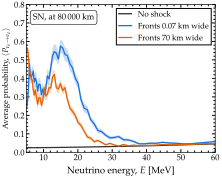
The shock signature against energy. Averaged \(\nu_e\) survival probability at the end of the ray of Figure A supernova shock front, at 80,000 km, without a shock and with the two front widths of that figure. With a shock, each point is the mean over a \(\pm\)10% energy window, which is what average=True returns when fronts are declared; the bands are the standard errors of those means. Without a shock, the passage is adiabatic, and the probability stays at a few percent. With one, it rises between 5 and about 25 MeV, where the resonance of the pair split by \(\Delta m^2_{31}\) lies at or near the forward shock. Above 30 MeV, the resonance lies in undisturbed matter, and the probability falls back toward the no-shock value. See notebooks #14 and #28.
Figure The shock signature against energy shows the effect of the shock on the energy spectrum. Without a shock, the passage is adiabatic, a \(\nu_e\) leaves as \(\nu_3\), and the survival probability is a few percent at all energies. With a shock, it rises to tens of percent between 5 and about 25 MeV. The window is set by where the resonance density, which falls as \(1/E\), sits on the profile. Between 1.8 and 18 MeV, the resonance density lies within the jump at the forward shock, so the resonance is crossed at the front. Above 18 MeV, it lies beyond the front, in undisturbed matter, where the crossing is adiabatic; the jump still changes the mixing angle, but less at higher energy, so the effect fades. Between 5.3 and 13 MeV, the resonance density also lies within the jump at the contact discontinuity. The resonance is then crossed at both fronts, and the result depends on the phase accumulated between them. Across most of the window, the sharp fronts give the larger probability: the oscillation length at the resonance, 20 to 60 km between 6 and 18 MeV, is comparable to the 70-km ramp, so the state partly follows the wide fronts. Near 5 MeV, the wide fronts give the larger probability.